Heat equation
In this example, we numerically solve the 1D heat equation
\[\frac{∂θ}{∂t} = ν \frac{∂^2 θ}{∂x^2},\]
in a bounded domain $x ∈ [-1, 1]$ with homogeneous Neumann boundary conditions, $∂_x θ(±1, t) = 0$.
Defining a B-spline basis
The general idea is to approximate the unknown solution by a spline of order $k$. For this, we first define a B-spline basis $\{ b_i(x), \, i = 1, …, N \}$, such that the solution at a given time $t$ is approximated by
\[θ(x, t) = ∑_{i = 1}^N v_i(t) b_i(x),\]
where the $v_i$ are the B-spline coefficients.
A B-spline basis is uniquely defined by its order $k$ and by a choice of knot locations within the spatial domain, which form the spatial grid.
For this example, we take a uniform repartition of knots in $[-1, 1]$.
knots_in = range(-1, 1; length = 11)-1.0:0.2:1.0We then create a B-spline basis of order $k = 4$ using these knots.
using BSplineKit
B = BSplineBasis(BSplineOrder(4), knots_in)
13-element BSplineBasis of order 4, domain [-1.0, 1.0]
knots: [-1.0, -1.0, -1.0, -1.0, -0.8, -0.6, -0.4, -0.2, 0.0, 0.2, 0.4, 0.6, 0.8, 1.0, 1.0, 1.0, 1.0]Note that the generated basis includes an augmented set of knots, in which each boundary is repeated $k$ times:
knots(B)17-element BSplineKit.BSplines.AugmentedKnots{Float64, 4, StepRangeLen{Float64, Base.TwicePrecision{Float64}, Base.TwicePrecision{Float64}, Int64}}:
-1.0
-1.0
-1.0
-1.0
-0.8
-0.6
-0.4
-0.2
0.0
0.2
0.4
0.6
0.8
1.0
1.0
1.0
1.0In other words, the boundary knots have multiplicity $k$, while interior knots have multiplicity 1. This is common practice in bounded domains, and translates the fact that the solution does not need to be continuous at the boundaries. This provides additional degrees of freedom notably for the boundary conditions. This behaviour can be disabled via the augment argument of BSplineBasis.
We can now plot the knot locations (crosses) and the generated B-spline basis:
using CairoMakie
using LaTeXStrings
CairoMakie.activate!(type = "svg", pt_per_unit = 2.0)

function plot_knots!(ax, ts; knot_offset = 0.05, kws...)
    ys = zero(ts)
    # Add offset to distinguish knots with multiplicity > 1
    for i in eachindex(ts)[(begin + 1):end]
        if ts[i] == ts[i - 1]
            ys[i] = ys[i - 1] + knot_offset
        end
    end
    scatter!(ax, ts, ys; marker = '×', markersize = 24, color = :gray, kws...)
    ax
end

function plot_basis!(ax, B; eval_args = (), kws...)
    cmap = cgrad(:tab20)
    N = length(B)
    ts = knots(B)
    hlines!(ax, 0; color = :gray)
    for (n, bi) in enumerate(B)
        color = cmap[(n - 1) / (N - 1)]
        i, j = extrema(support(bi))
        lines!(ax, ts[i]..ts[j], x -> bi(x, eval_args...); color, linewidth = 2.5)
    end
    plot_knots!(ax, ts; kws...)
    ax
end

fig = Figure()
ax = Axis(
    fig[1, 1];
    xlabel = rich("x"; font = :italic),
    ylabel = rich("b", subscript("i"), rich("(x)"; offset = (0.1, 0.0)); font = :italic),
)
plot_basis!(ax, B)
fig
Imposing boundary conditions
In BSplineKit, the recommended approach for solving boundary value problems is to use the basis recombination method. That is, to expand the solution onto a new basis consisting on linear combinations of B-splines $b_i(x)$, such that each recombined basis function $ϕ_j(x)$ individually satisfies the required homogeneous boundary conditions (BCs). Thanks to the local support of B-splines, basis recombination only involves a small number of B-splines near the boundaries.
Using the RecombinedBSplineBasis type, we can easily define such recombined bases for many different BCs. In this example we generate a basis satisfying homogeneous Neumann BCs:
R = RecombinedBSplineBasis(B, Derivative(1))

fig = Figure()
ax = Axis(
    fig[1, 1];
    xlabel = rich("x"; font = :italic),
    ylabel = rich("ϕ", subscript("i"), rich("(x)"; offset = (0.1, 0.0)); font = :italic),
)
plot_basis!(ax, R)
fig
We notice that, on each of the two boundaries, the two initial (or final) B-splines of the original basis have been combined to produce a single basis function that has zero derivative at each respective boundary. To verify this, we can plot the basis function derivatives:
fig = Figure()
ax = Axis(
    fig[1, 1];
    xlabel = rich("x"; font = :italic),
    ylabel = rich("ϕ′", subscript("i"; offset = (-0.3, 0.0)), rich("(x)"; offset = (0.1, 0.0)); font = :italic),
)
plot_basis!(ax, R; eval_args = (Derivative(1), ), knot_offset = 0.4)
fig
Note that the new basis has two less functions than the original one, reflecting a loss of two degrees of freedom corresponding to the new constraints on each boundary:
length(B), length(R)(13, 11)Recombination matrix
As stated above, the basis recombination approach consists in performing linear combinations of B-splines $b_i$ to obtain a derived basis of functions $ϕ_j$ satisfying certain boundary conditions. This can be conveniently expressed using a transformation matrix $\mathbf{T}$ relating the two bases:
\[ϕ_j(x) = ∑_{i = 1}^N T_{ij} b_i(x) \quad \text{for } j = 1, 2, …, M,\]
where $N$ is the number of B-splines $b_i$, and $M < N$ is the number of $ϕ_j$ functions (in this example, $M = N - 2$).
The recombination matrix associated to the generated basis can be obtained using recombination_matrix:
T = recombination_matrix(R)13×11 RecombineMatrix{Bool, Pair{Tuple{Derivative{1}}, StaticArraysCore.SMatrix{2, 1, Bool, 2}}, Pair{Tuple{Derivative{1}}, StaticArraysCore.SMatrix{2, 1, Bool, 2}}}:
1 ⋅ ⋅ ⋅ ⋅ ⋅ ⋅ ⋅ ⋅ ⋅ ⋅
1 ⋅ ⋅ ⋅ ⋅ ⋅ ⋅ ⋅ ⋅ ⋅ ⋅
⋅ 1 ⋅ ⋅ ⋅ ⋅ ⋅ ⋅ ⋅ ⋅ ⋅
⋅ ⋅ 1 ⋅ ⋅ ⋅ ⋅ ⋅ ⋅ ⋅ ⋅
⋅ ⋅ ⋅ 1 ⋅ ⋅ ⋅ ⋅ ⋅ ⋅ ⋅
⋅ ⋅ ⋅ ⋅ 1 ⋅ ⋅ ⋅ ⋅ ⋅ ⋅
⋅ ⋅ ⋅ ⋅ ⋅ 1 ⋅ ⋅ ⋅ ⋅ ⋅
⋅ ⋅ ⋅ ⋅ ⋅ ⋅ 1 ⋅ ⋅ ⋅ ⋅
⋅ ⋅ ⋅ ⋅ ⋅ ⋅ ⋅ 1 ⋅ ⋅ ⋅
⋅ ⋅ ⋅ ⋅ ⋅ ⋅ ⋅ ⋅ 1 ⋅ ⋅
⋅ ⋅ ⋅ ⋅ ⋅ ⋅ ⋅ ⋅ ⋅ 1 ⋅
⋅ ⋅ ⋅ ⋅ ⋅ ⋅ ⋅ ⋅ ⋅ ⋅ 1
⋅ ⋅ ⋅ ⋅ ⋅ ⋅ ⋅ ⋅ ⋅ ⋅ 1Note that the matrix is almost an identity matrix, since most B-splines are kept intact in the new basis. This simple structure allows for very efficient computations using this matrix. The first and last columns indicate that Neumann BCs are imposed by adding the two first (and two last) B-splines, i.e.
\[ϕ_1(x) = b_1(x) + b_2(x), \qquad ϕ_M(x) = b_{N - 1}(x) + b_N(x).\]
Representation of the solution
Note that the solution $θ(x, t)$ can be represented in the original and in the recombined B-spline bases as
\[θ(x, t) = ∑_{i = 1}^N v_i(t) b_i(x) = ∑_{j = 1}^M u_j(t) ϕ_j(x),\]
where the $u_j$ are the coefficients in the recombined basis.
The recombination matrix introduced above can be used to transform between the coefficients $u_j$ and $v_i$ in both bases, via the linear relation $\bm{v} = \mathbf{T} \bm{u}$.
Initial condition
We come back now to our problem. We want to impose the following initial condition:
\[θ(x, 0) = θ_0(x) = 1 + \cos(π x).\]
First, we approximate this initial condition in the recombined B-spline basis that we have just constructed. This may be easily done using approximate:
θ₀(x) = 1 + cos(π * x)
θ₀_spline = approximate(θ₀, R, MinimiseL2Error())
SplineApproximation containing the 11-element Spline{Float64}:
basis: 11-element RecombinedBSplineBasis of order 4, domain [-1.0, 1.0], BCs {left => (D{1},), right => (D{1},)}
order: 4
knots: [-1.0, -1.0, -1.0, -1.0, -0.8, -0.6, -0.4, -0.2, 0.0, 0.2, 0.4, 0.6, 0.8, 1.0, 1.0, 1.0, 1.0]
coefficients: [-0.000237504, 0.135773, 0.669895, 1.33011, 1.86423, 2.06824, 1.86423, 1.33011, 0.669895, 0.135773, -0.000237504]
approximation method: MinimiseL2Error()To see that everything went well, we can plot the exact initial condition and its spline approximation, which show no important differences.
fig = Figure(size = (800, 400))
let ax = Axis(fig[1, 1]; xlabel = rich("x"; font = :italic), ylabel = rich("θ"; font = :italic))
    lines!(ax, -1..1, θ₀; label = rich("θ", subscript("0"), rich("(x)"; offset = (0.1, 0.0)); font = :italic), color = :blue)
    lines!(ax, -1..1, θ₀_spline; label = "Approximation", color = :orange, linestyle = :dash)
    axislegend(ax; position = :cb)
end
let ax = Axis(fig[1, 2]; xlabel = rich("x"; font = :italic), ylabel = "Difference")
    lines!(ax, -1..1, x -> θ₀(x) - θ₀_spline(x))
    plot_knots!(ax, knots(R); knot_offset = 0)
end
fig
Note that we have access to the recombined B-spline coefficients $u_j$ associated to the initial condition, which we will use further below:
u_init = coefficients(θ₀_spline)11-element Vector{Float64}:
-0.00023750401824749234
0.13577332485095295
0.6698947840773806
1.3301052159226192
1.8642266751490482
2.0682429184528472
1.8642266751490455
1.3301052159226219
0.6698947840773782
0.13577332485095484
-0.00023750401824791596Solving the heat equation
To solve the governing equation, the strategy is to project the unknown solution onto the chosen recombined basis. That is, we approximate the solution as
\[θ(x, t) = \sum_{j = 1}^M u_j(t) \, ϕ_j(x).\]
Plugging this representation into the heat equation, we find
\[\newcommand{\dd}{\mathrm{d}} ∑_j \frac{\dd u_j}{\dd t} \, ϕ_j(x) = ν ∑_j u_j \, ϕ_j''(x),\]
where primes denote spatial derivatives.
We can now use the method of mean weighted residuals to find the coefficients $u_j$, by projecting the above equation onto a chosen set of test functions $φ_i$:
\[∑_j \frac{\mathrm{d} u_j}{\mathrm{d} t} \, ⟨φ_i, ϕ_j⟩ = ν ∑_j u_j \, ⟨φ_i, ϕ_j''⟩,\]
where $⟨ f, g ⟩ = ∫_{-1}^1 f(x) \, g(x) \, \mathrm{d} x$ is the inner product between functions.
By choosing $M$ different test functions $φ_i$, the above problem can be written as the linear system
\[\mathbf{A} \frac{\mathrm{d} \bm{u}(t)}{\mathrm{d} t} = ν \mathbf{L} \bm{u}(t),\]
where the matrices are defined by $A_{ij} = ⟨ φ_i, ϕ_j ⟩$ and $L_{ij} = ⟨ φ_i, ϕ_j'' ⟩$.
Two of the most common choices of test functions $φ_i$ are:
$φ_i(x) = δ(x - x_i)$, where $δ$ is Dirac's delta, and $x_i$ are a set of collocation points where the equation will be satisfied. This approach is known as the collocation method.
$φ_i(x) = ϕ_i(x)$, in which case this is the Galerkin method.
We describe the solution using both methods in the following.
Collocation method
For the collocation method, we need to choose a set of $M$ grid points $x_j$. Since the basis functions implicitly satisfy the boundary conditions, these points must be chosen inside of the domain.
The collocation points may be automatically generated by calling collocation_points. Note that, since we pass the recombined basis R, the boundaries are not included in the chosen points:
xcol = collocation_points(R)11-element Vector{Float64}:
-0.9333333333333332
-0.7999999999999999
-0.6
-0.39999999999999997
-0.19999999999999998
1.850371707708594e-17
0.20000000000000004
0.4000000000000001
0.6
0.7999999999999999
0.9333333333333332We can now construct the matrices $\mathbf{A}$ and $\mathbf{L}$ associated to the collocation method. By definition, these matrices simply contain the evaluations of all basis functions $ϕ_j$ and their derivatives at the collocation points: $A_{ij} = ϕ_j(x_i)$ and $L_{ij} = ϕ_j''(x_i)$. Both these matrices can be constructed in BSplineKit using collocation_matrix. Note that both matrices are of type CollocationMatrix, which wrap matrices defined in BandedMatrices.jl.
Acol = collocation_matrix(R, xcol)
Lcol = collocation_matrix(R, xcol, Derivative(2))
11×11 CollocationMatrix{Float64} with bandwidths (2, 2):
-37.5 29.1667 8.33333 … 0.0 0.0 0.0
37.5 -62.5 25.0 0.0 0.0 0.0
0.0 25.0 -50.0 0.0 0.0 0.0
0.0 0.0 25.0 0.0 0.0 0.0
0.0 0.0 0.0 0.0 0.0 0.0
0.0 0.0 0.0 … 0.0 0.0 0.0
0.0 0.0 0.0 3.46945e-15 0.0 0.0
0.0 0.0 0.0 25.0 6.93889e-15 0.0
0.0 0.0 0.0 -50.0 25.0 0.0
0.0 0.0 0.0 25.0 -62.5 37.5
0.0 0.0 0.0 … 8.33333 29.1667 -37.5For convenience and performance, we can incorporate the heat diffusivity $ν$ in the $\mathbf{L}$ matrix:
ν = 0.01
Lcol *= ν
11×11 BandedMatrix{Float64} with bandwidths (2, 2):
-0.375 0.291667 0.0833333 … ⋅ ⋅ ⋅
0.375 -0.625 0.25 ⋅ ⋅ ⋅
0.0 0.25 -0.5 ⋅ ⋅ ⋅
⋅ 0.0 0.25 ⋅ ⋅ ⋅
⋅ ⋅ 0.0 ⋅ ⋅ ⋅
⋅ ⋅ ⋅ … ⋅ ⋅ ⋅
⋅ ⋅ ⋅ 3.46945e-17 ⋅ ⋅
⋅ ⋅ ⋅ 0.25 6.93889e-17 ⋅
⋅ ⋅ ⋅ -0.5 0.25 0.0
⋅ ⋅ ⋅ 0.25 -0.625 0.375
⋅ ⋅ ⋅ … 0.0833333 0.291667 -0.375Finally, for the time integration, we use OrdinaryDiffEqTsit5.jl from the DifferentialEquations.jl suite.
using LinearAlgebra
using OrdinaryDiffEqTsit5

function heat_rhs!(du, u, params, t)
    mul!(du, params.L, u)    # du = ν * L * u
    ldiv!(du, params.A, du)  # du = A \ (ν * L * u)
    du
end

# Solver parameters
params_col = (
    A = lu(Acol),  # we pass the factorised matrix A for performance
    L = Lcol,
)

tspan = (0.0, 10.0)
prob = ODEProblem(heat_rhs!, u_init, tspan, params_col)
prob = ODEProblem{true}(heat_rhs!, u_init, tspan, params_col)
sol_collocation = solve(prob, Tsit5(); saveat = 0.5)

function plot_heat_solution(sol, R)
    fig = Figure()
    ax = Axis(fig[1, 1]; xlabel = rich("x"; font = :italic), ylabel = rich("θ(x,t)"; font = :italic))
    colormap = cgrad(:viridis)
    tspan = sol.prob.tspan
    Δt = tspan[2] - tspan[1]
    for (u, t) in tuples(sol)
        S = Spline(R, u)
        color = colormap[(t - tspan[1]) / Δt]
        lines!(ax, -1..1, S; label = string(t), color, linewidth = 2)
    end
    Colorbar(fig[1, 2]; colormap, limits = tspan, label = "Time")
    fig
end

# NOTE: there's an issue in CairoMakie 0.11.10 when saving SVGs with colourbars, so we fall
# back to PNG output.
# See https://github.com/MakieOrg/Makie.jl/issues/3016
CairoMakie.activate!(type = "png", px_per_unit = 2.0)
plot_heat_solution(sol_collocation, R)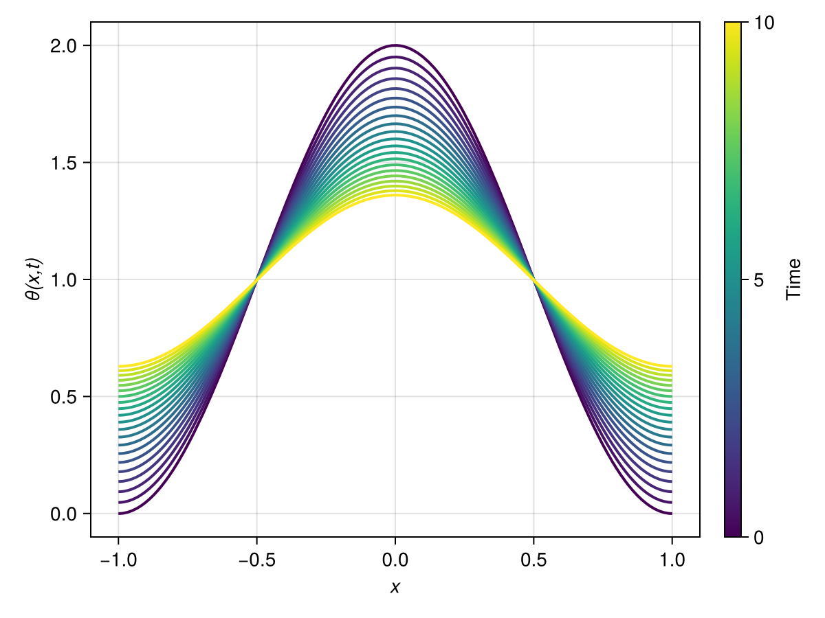
Galerkin method
We start by constructing the Galerkin matrices $\mathbf{A}$ and $\mathbf{L}$. The first of these matrices, $A_{ij} = ⟨ ϕ_i, ϕ_j ⟩$, is usually known as the mass matrix of the system. It is a positive definite symmetric matrix, which enables the use of Cholesky factorisation to solve the resulting linear system. Moreover, here it is banded thanks to the local support of the B-splines. The mass matrix can be constructed by calling galerkin_matrix:
Agal = galerkin_matrix(R)11×11 LinearAlgebra.Hermitian{Float64, BandedMatrices.BandedMatrix{Float64, Matrix{Float64}, Base.OneTo{Int64}}}:
0.107857 0.0349405 0.00714286 … ⋅ ⋅ ⋅
0.0349405 0.0653571 0.0449206 ⋅ ⋅ ⋅
0.00714286 0.0449206 0.095873 ⋅ ⋅ ⋅
5.95238e-5 0.00474206 0.0472619 ⋅ ⋅ ⋅
⋅ 3.96825e-5 0.0047619 ⋅ ⋅ ⋅
⋅ ⋅ 3.96825e-5 … 3.96825e-5 ⋅ ⋅
⋅ ⋅ ⋅ 0.0047619 3.96825e-5 ⋅
⋅ ⋅ ⋅ 0.0472619 0.00474206 5.95238e-5
⋅ ⋅ ⋅ 0.095873 0.0449206 0.00714286
⋅ ⋅ ⋅ 0.0449206 0.0653571 0.0349405
⋅ ⋅ ⋅ … 0.00714286 0.0349405 0.107857Note that, unlike the collocation method, in the Galerkin method we don't need to specify a set of grid points, as functions are not evaluated at collocation points (they are instead integrated over the whole domain). The integration is performed using Gauss–Legendre quadrature, which can be made exact up to numerical precision, taking advantage of the fact that the product of two B-splines is a piecewise polynomial.
As for the matrix $\mathbf{L}$ representing the second derivative operator, we can write it using integration by parts as
\[L_{ij} = ⟨ ϕ_i, ϕ_j'' ⟩ = -⟨ ϕ_i', ϕ_j' ⟩ + \left[ ϕ_i ϕ_j' \right]_{-1}^1 = -R_{ij},\]
where $R_{ij} = ⟨ ϕ_i', ϕ_j' ⟩$ is a positive definite symmetric matrix. Note that the boundary terms all vanish since all basis functions individually satisfy homogeneous Neumann boundary conditions, $ϕ_i'(±1) = 0$. (The same result would be obtained with homogeneous Dirichlet boundary conditions.)
As can be seen above, one well-known advantage of the Galerkin method is that the basis functions can satisfy weaker continuity conditions than in the collocation method, as high-order derivatives can be reduced using integration by parts.
The matrix $\mathbf{R}$ can be constructed using galerkin_matrix:
Rgal = galerkin_matrix(R, (Derivative(1), Derivative(1)))11×11 LinearAlgebra.Hermitian{Float64, BandedMatrices.BandedMatrix{Float64, Matrix{Float64}, Base.OneTo{Int64}}}:
3.75 -2.1875 -1.5 … ⋅ ⋅ ⋅
-2.1875 3.375 -0.166667 ⋅ ⋅ ⋅
-1.5 -0.166667 3.33333 ⋅ ⋅ ⋅
-0.0625 -0.979167 -0.625 ⋅ ⋅ ⋅
⋅ -0.0416667 -1.0 ⋅ ⋅ ⋅
⋅ ⋅ -0.0416667 … -0.0416667 ⋅ ⋅
⋅ ⋅ ⋅ -1.0 -0.0416667 ⋅
⋅ ⋅ ⋅ -0.625 -0.979167 -0.0625
⋅ ⋅ ⋅ 3.33333 -0.166667 -1.5
⋅ ⋅ ⋅ -0.166667 3.375 -2.1875
⋅ ⋅ ⋅ … -1.5 -2.1875 3.75Note that, instead, we could have constructed the original matrix $\mathbf{L}$, which, as expected, is equal to $\mathbf{R}$ up to a sign:
Lgal = galerkin_matrix(R, (Derivative(0), Derivative(2)))11×11 BandedMatrix{Float64} with bandwidths (3, 3):
-3.75 2.1875 1.5 … ⋅ ⋅ ⋅
2.1875 -3.375 0.166667 ⋅ ⋅ ⋅
1.5 0.166667 -3.33333 ⋅ ⋅ ⋅
0.0625 0.979167 0.625 ⋅ ⋅ ⋅
⋅ 0.0416667 1.0 ⋅ ⋅ ⋅
⋅ ⋅ 0.0416667 … 0.0416667 ⋅ ⋅
⋅ ⋅ ⋅ 1.0 0.0416667 ⋅
⋅ ⋅ ⋅ 0.625 0.979167 0.0625
⋅ ⋅ ⋅ -3.33333 0.166667 1.5
⋅ ⋅ ⋅ 0.166667 -3.375 2.1875
⋅ ⋅ ⋅ … 1.5 2.1875 -3.75As in the collocation example, we include the heat diffusivity $ν$ in the $\mathbf{R}$ matrix:
parent(Rgal) .*= -ν # we can't directly multiply Rgal, as it's a Hermitian wrapper11×11 BandedMatrix{Float64} with bandwidths (0, 3):
-0.0375 0.021875 0.015 0.000625 … ⋅ ⋅
⋅ -0.03375 0.00166667 0.00979167 ⋅ ⋅
⋅ ⋅ -0.0333333 0.00625 ⋅ ⋅
⋅ ⋅ ⋅ -0.0333333 ⋅ ⋅
⋅ ⋅ ⋅ ⋅ ⋅ ⋅
⋅ ⋅ ⋅ ⋅ … ⋅ ⋅
⋅ ⋅ ⋅ ⋅ 0.000416667 ⋅
⋅ ⋅ ⋅ ⋅ 0.00979167 0.000625
⋅ ⋅ ⋅ ⋅ 0.00166667 0.015
⋅ ⋅ ⋅ ⋅ -0.03375 0.021875
⋅ ⋅ ⋅ ⋅ … ⋅ -0.0375We finally solve using DifferentialEquations.jl. Note that not much is changed compared to the collocation example. The only difference is that we use a Cholesky factorisation for the mass matrix $\mathbf{A}$.
params_gal = (
    A = cholesky(Agal),
    L = Rgal,
)

prob = ODEProblem{true}(heat_rhs!, u_init, tspan, params_gal)
sol_galerkin = solve(prob, Tsit5(); saveat = 0.5)

plot_heat_solution(sol_galerkin, R)
Result comparison
The solution of the Galerkin method looks very similar to the one obtained with the collocation method. However, as seen below, there are non-negligible differences between the two.
fig = Figure(size = (800, 400))
let ax = Axis(fig[1, 1]; xlabel = rich("x"; font = :italic), ylabel = rich("θ(x, t = $(tspan[end]))"; font = :italic))
    for pair in (
            "Collocation" => sol_collocation,
            "Galerkin" => sol_galerkin,
        )
        label, sol = pair
        u = last(sol.u)
        S = Spline(R, u)
        lines!(ax, -1..1, S; label, linewidth = 2)
    end
    axislegend(ax; position = :cb)
end
let ax = Axis(fig[1, 2]; xlabel = rich("x"; font = :italic), ylabel = "Difference")
    Sc = Spline(R, last(sol_collocation.u))
    Sg = Spline(R, last(sol_galerkin.u))
    lines!(ax, -1..1, x -> Sc(x) - Sg(x); linewidth = 2)
end
fig
Compared to the Galerkin method, there seems to be some additional dissipation in the domain interior when using the collocation method. This hints at the presence of numerical dissipation introduced by this method.
To finish, we compare the two solutions to a solution at a higher resolution, using a higher number of B-spline knots and a higher B-spline order. This last solution is obtained using the collocation method to allow for better comparisons between both methods.
hi_res = let
    knots_in = range(-1, 1; length = 101)
    B = BSplineBasis(BSplineOrder(6), knots_in)
    R = RecombinedBSplineBasis(B, Derivative(1))
    θ₀_spline = approximate(θ₀, R)
    u_init = coefficients(θ₀_spline)
    xcol = collocation_points(R)
    Acol = collocation_matrix(R, xcol)
    Lcol = ν .* collocation_matrix(R, xcol, Derivative(2))
    params_col = (A = lu(Acol), L = Lcol)
    prob = ODEProblem{true}(heat_rhs!, u_init, tspan, params_col)
    sol = solve(prob, Tsit5(); saveat = 0.5)
    (; R, sol)
end

fig = Figure(size = (800, 400))
let ax = Axis(fig[1, 1])
    ax.xlabel = rich("x"; font = :italic)
    ax.ylabel = rich("θ(x, t = $(tspan[end]))"; font = :italic)
    for pair in (
            "Collocation" => sol_collocation,
            "Galerkin" => sol_galerkin,
        )
        label, sol = pair
        u = last(sol.u)
        S = Spline(R, u)
        lines!(ax, -1..1, S; label, linewidth = 2)
    end
    let u = last(hi_res.sol.u)
        S = Spline(hi_res.R, u)
        lines!(ax, -1..1, S; label = "Hi-res", linewidth = 2, linestyle = :dash, color = :gray)
    end
    axislegend(ax; position = :cb)
end
let ax = Axis(fig[1, 2]; ylabel = "Difference with hi-res solution")
    ax.xlabel = rich("x"; font = :italic)
    Sc = Spline(R, last(sol_collocation.u))
    Sg = Spline(R, last(sol_galerkin.u))
    S_hi = Spline(hi_res.R, last(hi_res.sol.u))
    lines!(ax, -1..1, x -> Sc(x) - S_hi(x); label = rich("Collocation"), linewidth = 2)
    lines!(ax, -1..1, x -> Sg(x) - S_hi(x); label = rich("Galerkin"), linewidth = 2)
    axislegend(ax; position = :rb)
end
fig
We see that the low-resolution solution with the Galerkin method matches the high-resolution solution. This confirms that the Galerkin method provides higher accuracy than the collocation method when both are used at the same resolution.
This page was generated using Literate.jl.