Kelvin waves

This tutorial describes the simulation of Kelvin waves propagating along nearly-straight and infinite vortex lines.

Here we will:

• learn how to define infinite but unclosed filaments;

• look at diagnostics such as the energy over time;

• perform spatial and temporal Fourier analysis to detect relevant wavenumbers and frequencies associated to Kelvin waves.

It is recommended to first follow the vortex ring tutorial before following this tutorial.

Physical configuration

The idea of this tutorial is to study the time evolution of an infinite straight line slightly modified by a sinusoidal perturbation.

We will consider such a vortex line in a cubic periodic domain of size $L=2\pi$. The line is oriented in the $z$ direction and modified by a perturbation of amplitude $ϵL$ along $x$. The perturbation is periodic with period $\lambda =L/m=2\pi /m$ where $m$ is an integer representing the mode of the perturbation (relative to the domain size $L$).

Such an infinite line $\mathit{s}=(x,y,z)$ can be parametrised as

$$\begin{array}{rl}x(t)& =x_0+ϵ\sin (2\pi mt)\\ y(t)& =y_0\\ z(t)& =z_0+(t-\frac{1}{2})L\end{array}$$

for $t\in \mathbb{R}$. In particular, note that the line exactly crosses the domain after a period $T=1$, going from $\mathit{s}(t)$ to $\mathit{s}(t+1)=\mathit{s}(t)+(0,0,L)$.

The analytical prediction is that, over time, a small perturbation should rotate around the vortex in the direction opposite to its circulation. Its frequency is given by (see e.g. Schwarz (1985)):

$${\omega }_{\text{KW}}(k)=\frac{\Gamma k^2}{4\pi }[\ln \left(\frac{2}{ka}\right)-\gamma +\frac{1}{2}-\Delta ]$$

where $k=2\pi m/L$ is the perturbation wavenumber, $\gamma \approx 0.5772$ the Euler–Mascheroni constant, $\Delta$ the vortex core parameter and $a$ its radius ($a\ll 1/k$).

Defining an unclosed infinite curve

Following the vortex ring tutorial, one may want to define such a line as follows:

using VortexPasta
using VortexPasta.Filaments
using VortexPasta.Filaments: Vec3

N = 64  # number of discretisation points per line
m = 2    # perturbation mode
L = 2π   # domain period
x⃗₀ = Vec3(L/4, L/4, L/2)  # line "origin"
ϵ = 0.01
ts = range(0, 1; length = N + 1)[1:N]  # important: we exclude the endpoint (t = 1)
points = [x⃗₀ + Vec3(ϵ * L * sinpi(2m * t), 0, L * (t - 1/2)) for t ∈ ts]
f = Filaments.init(ClosedFilament, points, QuinticSplineMethod())

Let's look at the result:

using GLMakie

# Give a colour to a filament based on its local orientation wrt Z.
function filament_colour(f::AbstractFilament, refinement)
    cs = Float32[]
    ζs = range(0, 1; length = refinement + 1)[1:refinement]  # for interpolation
    for seg ∈ segments(f), ζ ∈ ζs
        colour = seg(ζ, UnitTangent())[3]  # in [-1, 1]
        push!(cs, colour)
    end
    let seg = last(segments(f))  # "close" the curve
        colour = seg(1.0, UnitTangent())[3]
        push!(cs, colour)
    end
    cs
end

# Plot a list of filaments
function plot_filaments(fs::AbstractVector)
    fig = Figure()
    ax = Axis3(fig[1, 1]; aspect = :data)
    ticks = range(0, 2π; step = π/2)
    tickformat(xs) = map(x -> string(x/π, "π"), xs)
    ax.xticks = ax.yticks = ax.zticks = ticks
    ax.xtickformat = ax.ytickformat = ax.ztickformat = tickformat
    hidespines!(ax)
    wireframe!(ax, Rect(0, 0, 0, L, L, L); color = (:black, 0.5), linewidth = 0.2)
    for f ∈ fs
        refinement = 4
        color = filament_colour(f, refinement)
        plot!(
            ax, f;
            refinement, color, colormap = :RdBu_9, colorrange = (-1, 1), markersize = 4,
        )
    end
    fig
end

# Plot a single filament
plot_filaments(f::AbstractFilament) = plot_filaments([f])

plot_filaments(f)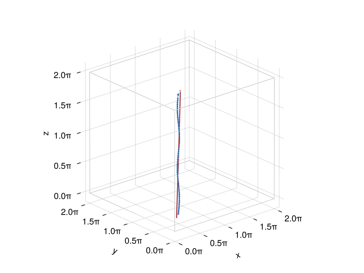

Things look almost as expected except for the fact that the line tries to close itself when it reaches the end. To avoid this, one needs to explicitly give Filaments.init an end-to-end vector via the offset keyword argument. In our case the end-to-end vector is $\mathit{\Delta }=(0,0,2\pi )$.

f = Filaments.init(ClosedFilament, points, QuinticSplineMethod(); offset = (0, 0, 2π))
plot_filaments(f)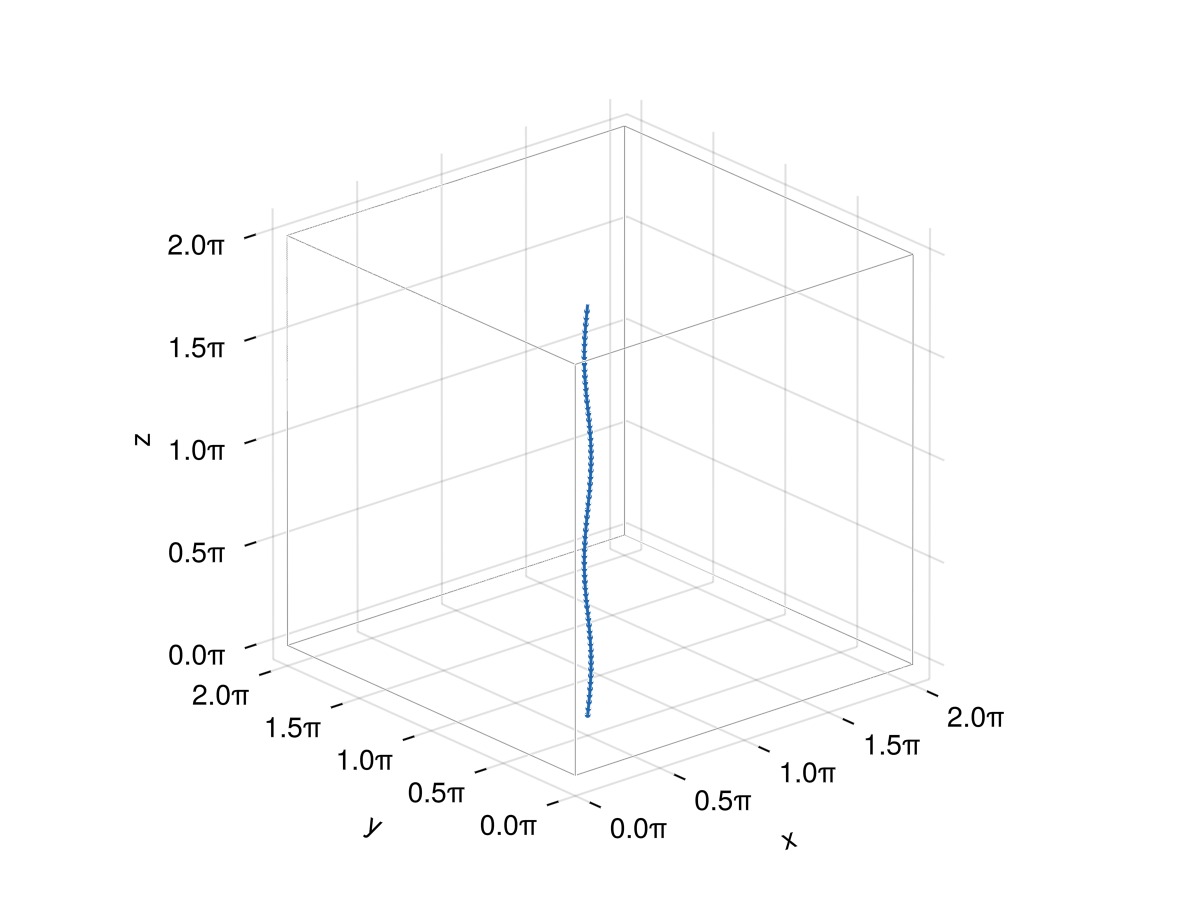

Now everything looks fine! Note that the end-to-end vector corresponds to the separation between a node f[i] and the node f[i + N]. For example:

@show f[end + 1] - f[begin]
@show Vec3(0, 0, 2π)

f[end + 1] - f[begin] = [0.0, 0.0, 6.283185307179586]
Vec3(0, 0, 2π) = [0.0, 0.0, 6.283185307179586]

End-to-end vector

The end-to-end vector must be an integer multiple of the domain period, which in this case is $(2\pi ,2\pi ,2\pi )$.

Defining a curve from parametric function

The Filaments.init function actually allows to define a curve directly from its (continuous) parametric function. In this case one doesn't need to care about end-to-end vectors and "offsets", since these are usually encoded in the parametrisation.

For example, for the curve above we would define the function:

fcurve(t) = x⃗₀ + Vec3(
    ϵ * L * sinpi(2 * m * t),
    0,
    (t - 0.5) * L,
)

fcurve (generic function with 1 method)

The function will be evaluated over the interval $t\in [0,1]$. The only assumption is that the parametric function must either represent:

• a closed curve with period $T=1$;

• an unclosed periodic curve which crosses the domain after a period $T=1$.

Here we are in the second case, and the function above indeed satisfies this condition.

Now we just pass the function to Filaments.init:

f_alt = Filaments.init(fcurve, ClosedFilament, N, QuinticSplineMethod())

Note that this generates a filament which is practically identical to the previous one (just with a shift in the node positions, not really visible here):

plot_filaments([f, f_alt])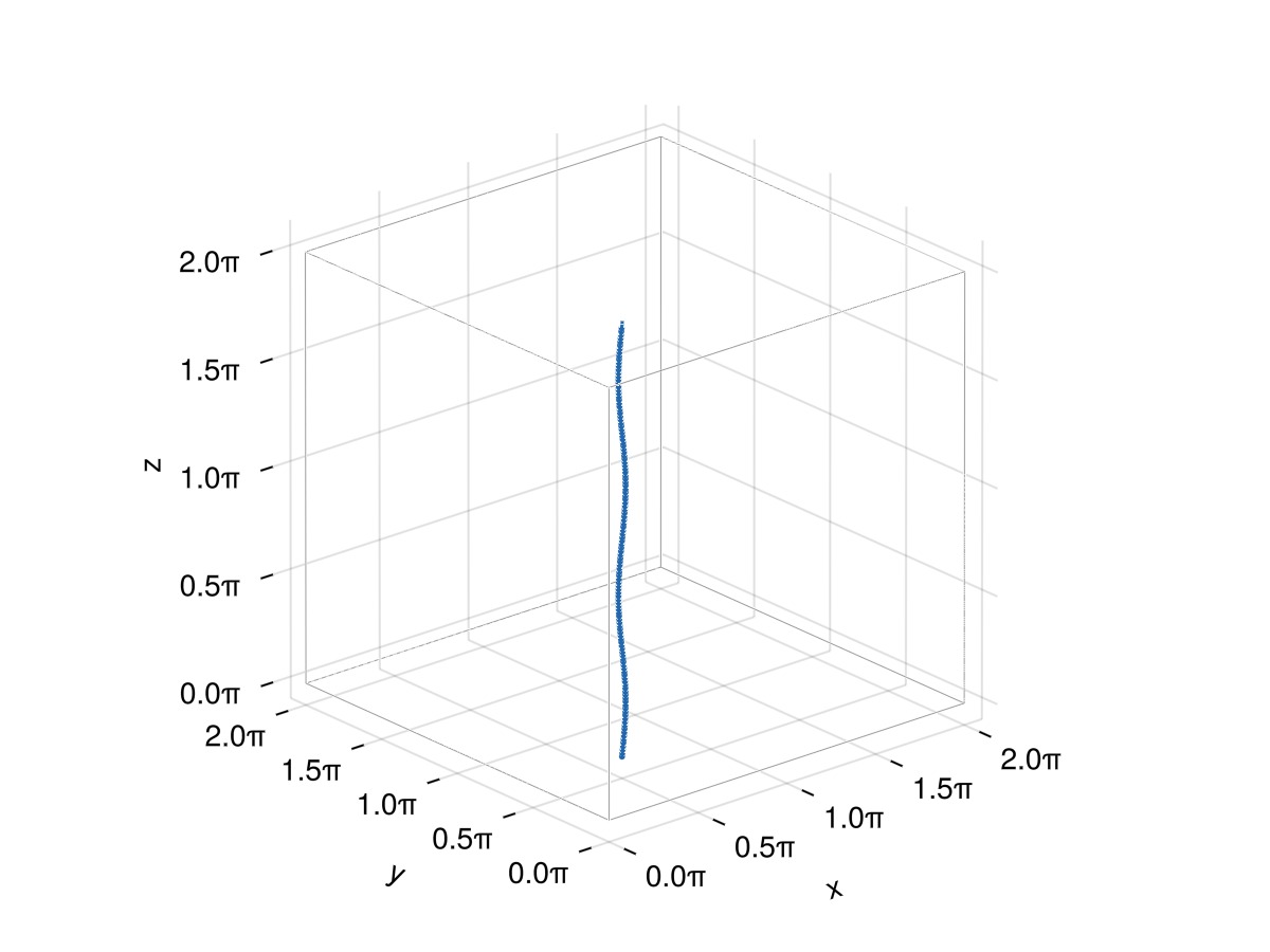

Using predefined curves

There is another convenient way of defining such curves, using the VortexPasta.PredefinedCurves module which provides definitions of parametric functions for commonly-used curves. As we will see in the next section, this is particularly convenient when we want to create multiple vortices which share the same geometry, but which have for instance different orientations or different spatial locations in the domain.

Here we want to use the PeriodicLine definitions, which allow one to pass arbitrary functions as perturbations. Note that curve definitions in PredefinedCurves are normalised. In particular, the period of PeriodicLine is 1, and the perturbation that we give it will be in terms of this unit period.

using VortexPasta.PredefinedCurves: PeriodicLine, define_curve
x_perturb(t) = ϵ * sinpi(2m * t)  # perturbation along x (takes t ∈ [0, 1])
p = PeriodicLine(x = x_perturb)   # this represents a line with period 1 along z

We now want to "convert" this line to a parametric function which can be then evaluated to generate points. This is done using the define_curve function, which allows in particular to rescale the curve (we want a period of $L=2\pi$ instead of $1$). We would also like the curve to be centred at ${\mathit{x}}_0$.

S = define_curve(p; scale = L, translate = x⃗₀)
@show S(0.0) S(0.5) S(1.0)

S(0.0) = [1.5707963267948966, 1.5707963267948966, 0.0]
S(0.5) = [1.5707963267948966, 1.5707963267948966, 3.141592653589793]
S(1.0) = [1.5707963267948966, 1.5707963267948966, 6.283185307179586]

As we can see, S is a function which can be evaluated at any value of $t$. In fact, S is identical to the fcurve function we defined above. We can now pass this function to Filaments.init to generate a filament:

f = Filaments.init(S, ClosedFilament, N, QuinticSplineMethod())
plot_filaments(f)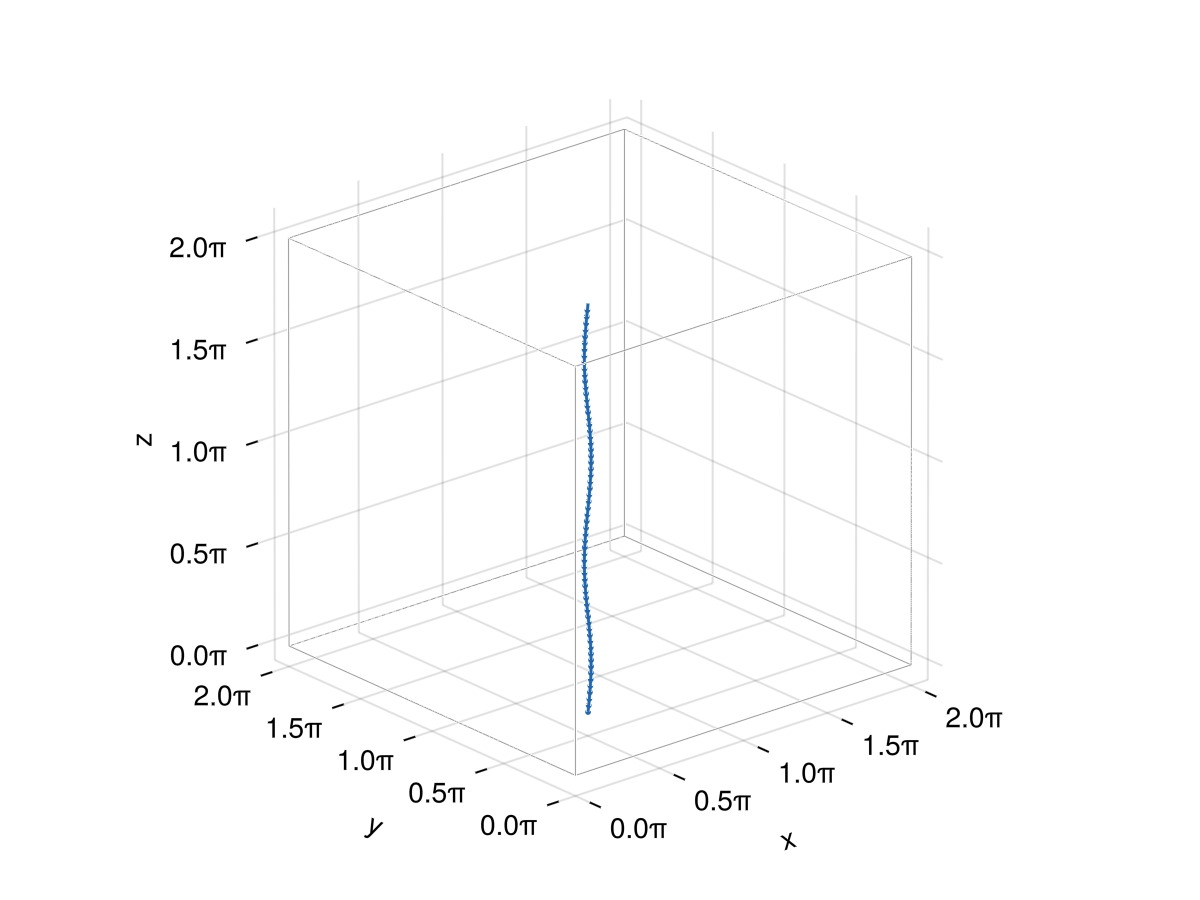

Ensuring periodicity of the velocity

For now we have initialised one infinite unclosed filament. One needs to be careful when working with unclosed filaments in periodic domains. Indeed, a single straight vortex filament in a periodic domain generates a non-zero circulation along the domain boundaries (or equivalently, a non-zero mean vorticity), which violates the periodicity condition. (One may compensate this by considering a uniform background vorticity field with opposite circulation, but this is outside of the scope of the tutorial.)

The mean vorticity in the periodic domain is given by

$$⟨\mathit{\omega }⟩=\frac{1}{V}{\int }_{\Omega }\mathit{\omega }(\mathit{x}){\mathrm{d}}^3\mathit{x}=\frac{\Gamma }{V}{\int }_{\mathcal{C}}\mathrm{d}\mathit{s}=\frac{\Gamma }{V}{\int }_{\mathcal{C}}{\mathit{s}}^{\prime }(t)\mathrm{d}t$$

where $\Omega$ represents the periodic domain and $V=L^3$ is its volume. So the last integral must be zero to ensure periodicity. It is quite obvious that this is not the case for the filament defined above, and we can readily verify it:

integrate(f_alt, GaussLegendre(4)) do ff, i, ζ
    ff(i, ζ, Derivative(1))
end

3-element SVector{3, Float64} with indices SOneTo(3):
 -6.765421556309548e-17
 -1.333667967889273e-29
  6.283185307179587

This means that, for each vortex oriented in the $+z$ direction, we need to compensate by a vortex oriented in the $-z$ direction to obtain a zero total circulation.

In practice, to make sure that the total circulation is zero and to stabilise the system, we want to have four vortices such that their coordinates respect mirror symmetry with respect to the planes $x=L/2$ and $y=L/2$. Respecting these two symmetries means that both planes effectively become impermeable (but free-slip) walls. That is, the velocity induced by the vortices on those planes can only be parallel to the planes and not normal to them. More generally, due to periodicity, all planes $x=nL/2$ and $y=nL/2$ (for integer $n$) effectively become impermeable walls.

Let's now create these four vortices:

funcs = [
    # "Positive" vortices
    define_curve(p; scale = (+L, +L, +L), translate = (0.25L, 0.25L, 0.5L)),
    define_curve(p; scale = (-L, -L, +L), translate = (0.75L, 0.75L, 0.5L)),  # mirror symmetry wrt x and y
    # "Negative" vortices: we use the `orientation` keyword to flip their orientation.
    define_curve(p; scale = (+L, -L, +L), translate = (0.25L, 0.75L, 0.5L), orientation = -1),  # mirror symmetry wrt y
    define_curve(p; scale = (-L, +L, +L), translate = (0.75L, 0.25L, 0.5L), orientation = -1),  # mirror symmetry wrt x
]
fs = [Filaments.init(S, ClosedFilament, N, QuinticSplineMethod()) for S in funcs]
plot_filaments(fs)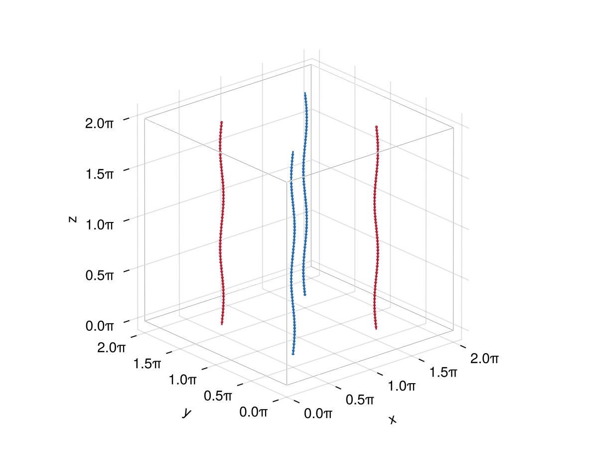

Here the colours represent the local orientation of the curve tangent with respect to the $z$ axis. We can check that, when we sum the contributions of all filaments, the mean vorticity is zero:

# This computes the integral along each filament and sums the results.
sum(fs) do f
    integrate(f, GaussLegendre(4)) do ff, i, ζ
        f(i, ζ, Derivative(1))
    end
end

3-element SVector{3, Float64} with indices SOneTo(3):
 -7.45931094670027e-17
 -2.7739554174998235e-29
  2.6645352591003757e-15

Now we're ready to perform simulations.

Simulating Kelvin waves

As in the vortex ring tutorial, we use the Timestepping module to perform a temporal simulation of the configuration we just prepared.

Setting physical and numerical parameters

We start by setting the parameters for Biot–Savart computations:

using VortexPasta.BiotSavart
M = floor(Int, 32 * 2/3)  # resolution of long-range grid
kmax = π * (M - 1) / L    # maximum resolved wavenumber (Nyquist frequency) for long-range part
β = 3.5                   # accuracy parameter
α = kmax / (2β)           # Ewald splitting parameter

params = ParamsBiotSavart(;
    Γ = 1.0,    # vortex circulation
    a = 1e-8,   # vortex core size
    Δ = 1/4,    # vortex core parameter (1/4 for a constant vorticity distribution)
    α = α,      # Ewald splitting parameter
    Ls = (L, L, L),  # same domain size in all directions
    Ns = (M, M, M),  # same long-range resolution in all directions
    rcut = β / α,    # cut-off distance for short-range computations
    quadrature = GaussLegendre(3),        # quadrature for integrals over filament segments
    backend_long = NonuniformFFTsBackend(),  # this is the default
    backend_short = CellListsBackend(2),
)

ParamsBiotSavart{Float64} with:
 - Physical parameters:
   * Vortex circulation:         Γ  = 1.0
   * Vortex core radius:         a  = 1.0e-8
   * Vortex core parameter:      Δ  = 0.25
   * Domain period:              Ls = (6.283185307179586, 6.283185307179586, 6.283185307179586)
 - Numerical parameters:
   * Ewald splitting parameter:  α = 1.4285714285714286 (σ = 1/α√2 = 0.49497474683058323)
   * Quadrature rule:            GaussLegendre{3}()
   * Quadrature rule (alt.):     GaussLegendre{3}() (used near singularities)
   * Avoid explicit erf:         true
   * Short-range backend:        CellListsBackend{2}(CPU(false); device = 1)
   * Short-range cut-off:        r_cut = 2.4499999999999997 (r_cut/L = 0.3899296105751435)
   * Short-range cut-off coeff.: β_shortrange = 3.4999999999999996
   * Local segment fraction:     1
   * Short-range uses SIMD:      true
   * Long-range backend:         NonuniformFFTsBackend(CPU(false); device = 1, m = HalfSupport(4), σ = 1.5)
   * Long-range resolution:      Ns = (21, 21, 21) (kmax = 10.0)
   * Long-range cut-off coeff.:  β_longrange = 3.5
   * Long-range spherical truncation: false

We would like to compute a few periods of Kelvin wave oscillations. For this, we first compute the expected Kelvin wave frequency and its associated period:

(; Γ, a, Δ,) = params         # extract parameters needed for KW frequency
γ = MathConstants.eulergamma  # Euler–Mascheroni constant
k = 2π * m / L
ω_kw = Γ * k^2 / (4 * π) * (
    log(2 / (k * a)) - γ + 1/2 - Δ
)
T_kw = 2π / ω_kw              # expected Kelvin wave period

1.0909579075062508

We create a VortexFilamentProblem to simulate a few Kelvin wave periods. To make things more interesting later when doing the temporal Fourier analysis of the results, we don't simulate an integer number of periods so that the results are not exactly time-periodic.

using VortexPasta.Timestepping
tspan = (0.0, 3.2 * T_kw)
prob = VortexFilamentProblem(fs, tspan, params)

VortexFilamentProblem with fields:
 ├─ p: ParamsBiotSavart{Float64}(Γ = 1.0, a = 1.0e-8, Δ = 0.25, α = 1.4285714285714286, …)
 ├─ tspan: (0.0, 3.491065304020003) -- simulation timespan
 └─ fs: 4-element VectorOfVectors -- vortex filaments at t = 0.0

We now create a callback which will be used to store some data for further analysis. We will store the times and the position over time of a single filament node to be able to visualise and analyse the oscillations. Moreover, we will store the system energy to verify that energy is conserved over time (see VFM notes for detains on how it is computed). For computing the energy we use the kinetic_energy_from_streamfunction function from the Diagnostics module.

using VortexPasta.Diagnostics

# We use `const` for performance reasons, as these variables are defined in global scope
# and used within the callback. If we were inside a function, these would not be needed
# (and in fact Julia complains if we use `const` inside a function).

const times = Float64[]
const X_probe = Vec3{Float64}[]  # will contain positions of a chosen node
const energy = Float64[]

# Save checkpoint file for visualisation every ≈ 0.1 * T_kw.
const t_checkpoint_step = 0.1 * T_kw
const t_checkpoint_next = Ref(tspan[1])  # save initial time, then every 0.1 * T_kw approx

function callback(iter)
    (; nstep, t,) = iter
    if nstep == 0  # make sure vectors are empty at the beginning of the simulation
        empty!(times)
        empty!(X_probe)
        empty!(energy)
        t_checkpoint_next[] = t
        # Remove VTKHDF files from a previous run
        for fname in readdir()
            if match(r"^kelvin_waves_(\d+)\.vtkhdf$", fname) !== nothing
                rm(fname)
            end
        end
    end
    push!(times, t)
    s⃗ = iter.fs[1][3]  # we choose a single node of a single filament
    push!(X_probe, s⃗)
    # Compute energy
    E = Diagnostics.kinetic_energy(iter)
    push!(energy, E)
    # Save VTKHDF file for visualisation
    if t ≥ t_checkpoint_next[]
        save_checkpoint("kelvin_waves_$(nstep).vtkhdf", iter)
        t_checkpoint_next[] += t_checkpoint_step  # time at which the next file will be saved
    end
    nothing
end

callback (generic function with 1 method)

Note that we have annotated the types of the variables times, X_probe and energy for performance reasons, since these are global variables which are used (and modified) from within the callback function. See here and here for details.

Choosing the timestep and the temporal scheme

In the vortex ring tutorial we have used the standard RK4 scheme. To capture the vortex evolution and avoid blow-up, this scheme requires the timestep $\Delta t$ to be of the order of the period of the fastest resolved Kelvin waves, which have a wavelength $\lambda$ equal to (twice) the filament resolution $\delta$ (the typical distance between two discretisation points).

We first estimate the filament resolution using minimum_node_distance:

δ = minimum_node_distance(prob.fs)  # should be close to L/N in our case

0.0981747704246807

Now we compute the Kelvin wave frequency associated to this distance:

kelvin_wave_period(λ; a, Δ, Γ) = 2 * λ^2 / Γ / (log(λ / (π * a)) + 1/2 - (Δ + MathConstants.γ))
dt_kw = kelvin_wave_period(δ; a, Δ, Γ)

0.0013178102262909038

Note that this time scale is very small compared to the period of the large-scale Kelvin waves:

T_kw / dt_kw

827.8566107176529

This means that we would need a relatively large simulation time to observe the evolution of large-scale Kelvin waves over multiple periods.

For the RK4 scheme, this time scale really seems to set the maximum allowed timestep limit. We can check that a simulation with RK4 using dt = dt_kw remains stable. In particular, energy stays constant in time after running a few iterations with this timestep:

iter = init(prob, RK4(); dt = dt_kw, callback)
for _ ∈ 1:40
    step!(iter)
end
energy'

1×41 adjoint(::Vector{Float64}) with eltype Float64:
 0.159397  0.159397  0.159397  0.159397  …  0.159397  0.159397  0.159397

However, using dt = 2 * dt_kw quickly leads to instability and energy blow-up:

iter = init(prob, RK4(); dt = 2 * dt_kw, callback)
for _ ∈ 1:40
    step!(iter)
end
energy'

1×41 adjoint(::Vector{Float64}) with eltype Float64:
 0.159397  0.159397  0.159397  0.159397  …  0.324634  0.322052  0.323562

This limit is basically set by the short-range Biot–Savart interactions and in particular the local term (see Desingularisation), which presents fast temporal variations. On the upside, this term is cheap to compute, which means that we can take advantage of a splitting scheme (such as Strang splitting) to accelerate computations.

The idea is to write the time evolution of a vortex point due to the Biot–Savart law as:

$$\frac{\mathrm{d}\mathit{s}}{\mathrm{d}t}=\mathit{v}(\mathit{s})={\mathit{v}}_{\text{local}}(\mathit{s})+{\mathit{v}}_{\text{non-local}}(\mathit{s})$$

where the local term ${\mathit{v}}_{\text{local}}(\mathit{s})$ represents the fast dynamics (thus requiring very small timesteps) while being cheap to compute, while the non-local term ${\mathit{v}}_{\text{non-local}}(\mathit{s})$ represents the slow dynamics and has a higher computational cost.

Using a splitting method can make sense when it is easier or more convenient to separately solve the two equations:

$$\begin{array}{rlrl}\frac{\mathrm{d}\mathit{s}}{\mathrm{d}t}& ={\mathit{v}}_{\text{local}}(\mathit{s})& & \text{(fast)}\\ \frac{\mathrm{d}\mathit{s}}{\mathrm{d}t}& ={\mathit{v}}_{\text{non-local}}(\mathit{s})& & \text{(slow)}\end{array}$$

In some applications, this is the case because one of the terms is linear or because one of the sub-equations can be solved analytically. This is not the case here, but this splitting is still convenient because it allows us to use different timesteps for each sub-equation. In particular, we can use a smaller timestep for the local (fast) term, which is the one that sets the timestep limit.

One of the most popular (and classical) splitting methods is Strang splitting, which is second order in time. In this method, a single simulation timestep ($t\to t+\Delta t$) is decomposed in 3 steps:

1. Advance solution $\mathit{s}(t)\to {\mathit{s}}_1$ in the interval $t\to t+\frac{\Delta t}{2}$ using equation $\text{(fast)}$.

2. Advance solution ${\mathit{s}}_1\to {\mathit{s}}_2$ in the interval $t\to t+\Delta t$ using equation $\text{(slow)}$.

3. Advance solution ${\mathit{s}}_2\to \mathit{s}(t+\Delta t)$ in the interval $t+\frac{\Delta t}{2}\to t+\Delta t$ using equation $\text{(fast)}$.

In the following we use the Strang splitting scheme, which allows to use different explicit Runge–Kutta schemes for the "fast" and "slow" equations, and allows to set a smaller timestep to solve the former.

Concretely, we solve steps 1 and 3 using the standard RK4 scheme, while for step 2 the Midpoint scheme is used by default (but this can be changed, see Strang docs for details). Moreover, steps 1 and 3 are decomposed into $M=16$ substeps, meaning that they are solved with a smaller timestep $\Delta t_{\text{fast}}=(\Delta t/2)/M=\Delta t/32$. In practice, this means that we can multiply our "global" timestep $\Delta t$ by 32 and retain the stability of the solver.

scheme = Strang(RK4(); nsubsteps = 16)
dt = 32 * dt_kw

0.04216992724130892

More generally, when using Strang splitting with the RK4 scheme for the fast dynamics, setting nsubsteps = M allows us to set the global timestep to dt = 2M * dt_kw. We could tune the number $M$ of inner iterations to allow even larger timesteps, but this might lead to precision loss.

Running the simulation

We now solve the full problem with this splitting scheme. Note that we use LocalTerm to identify the "fast" motions to the local (LIA) term of the Biot–Savart integrals. We could alternatively use ShortRangeTerm for a different interpretation of what represents the "fast" motions.

iter = init(prob, scheme; dt, callback, fast_term = LocalTerm())
reset_timer!(iter.to)  # to get more accurate timings (removes most of the compilation time)
solve!(iter)
iter.to

────────────────────────────────────────────────────────────────────────────────
                                       Time                    Allocations      
                              ───────────────────────   ────────────────────────
      Tot / % measured:            8.24s /  81.6%            481MiB /  62.5%    

Section               ncalls     time    %tot     avg     alloc    %tot      avg
────────────────────────────────────────────────────────────────────────────────
Update values at n...  10.9k    4.90s   72.8%   450μs    219MiB   72.9%  20.6KiB
  Biot-Savart (LIA...  10.6k    3.00s   44.6%   282μs    127MiB   42.2%  12.2KiB
    Add point charges  10.6k    1.74s   25.9%   164μs   45.2MiB   15.0%  4.35KiB
    Short-range co...  10.6k    1.02s   15.2%  96.4μs   52.6MiB   17.5%  5.07KiB
      Local term (...  10.6k    937ms   13.9%  88.2μs   22.7MiB    7.5%  2.19KiB
      Copy point c...  10.6k   46.1ms    0.7%  4.34μs   16.9MiB    5.6%  1.62KiB
      Synchronise GPU  10.6k    396μs    0.0%  37.3ns     0.00B    0.0%    0.00B
    Copy output (d...  10.6k   24.7ms    0.4%  2.33μs   2.43MiB    0.8%     240B
    Wait for async...  10.6k   2.36ms    0.0%   222ns     0.00B    0.0%    0.00B
  Biot-Savart (exc...    166    871ms   13.0%  5.25ms   23.5MiB    7.8%   145KiB
    Long-range com...    166    495ms    7.4%  2.98ms   14.7MiB    4.9%  90.5KiB
      Vorticity to...    166    268ms    4.0%  1.61ms   7.44MiB    2.5%  45.9KiB
      Interpolate ...    166    202ms    3.0%  1.22ms   6.00MiB    2.0%  37.0KiB
      Velocity fie...    166   22.1ms    0.3%   133μs    573KiB    0.2%  3.45KiB
      Copy point c...    166   1.29ms    0.0%  7.79μs    319KiB    0.1%  1.92KiB
      Process poin...    166    175μs    0.0%  1.05μs     0.00B    0.0%    0.00B
      Synchronise GPU    166   6.11μs    0.0%  36.8ns     0.00B    0.0%    0.00B
    Short-range co...    166    163ms    2.4%   982μs   2.03MiB    0.7%  12.5KiB
      Pair interac...    166    132ms    2.0%   795μs    416KiB    0.1%  2.51KiB
      Remove self-...    166   21.5ms    0.3%   129μs    397KiB    0.1%  2.39KiB
      Process poin...    166   6.54ms    0.1%  39.4μs    605KiB    0.2%  3.64KiB
      Copy point c...    166   1.80ms    0.0%  10.8μs    353KiB    0.1%  2.12KiB
      Synchronise GPU    166   6.45μs    0.0%  38.9ns     0.00B    0.0%    0.00B
    Add point charges    166   25.9ms    0.4%   156μs    724KiB    0.2%  4.36KiB
    Copy output (d...    332   1.26ms    0.0%  3.81μs    127KiB    0.0%     392B
    Wait for async...    332   85.3μs    0.0%   257ns     0.00B    0.0%    0.00B
    CPU-only opera...    166   14.0μs    0.0%  84.5ns     0.00B    0.0%    0.00B
  Biot-Savart (full)      83    482ms    7.2%  5.81ms   13.0MiB    4.3%   160KiB
    Long-range com...     83    367ms    5.5%  4.42ms   10.6MiB    3.5%   131KiB
      Interpolate ...    166    207ms    3.1%  1.25ms   5.99MiB    2.0%  37.0KiB
      Vorticity to...     83    138ms    2.1%  1.66ms   3.72MiB    1.2%  45.9KiB
      Velocity fie...     83   11.3ms    0.2%   136μs    287KiB    0.1%  3.45KiB
      Streamfuncti...     83   9.64ms    0.1%   116μs    287KiB    0.1%  3.45KiB
      Copy point c...     83    593μs    0.0%  7.15μs    160KiB    0.1%  1.92KiB
      Process poin...     83   95.4μs    0.0%  1.15μs     0.00B    0.0%    0.00B
      Synchronise GPU     83   3.05μs    0.0%  36.8ns     0.00B    0.0%    0.00B
    Short-range co...     83   93.4ms    1.4%  1.13ms   1.38MiB    0.5%  17.1KiB
      Pair interac...     83   67.4ms    1.0%   812μs    220KiB    0.1%  2.66KiB
      Remove self-...     83   11.2ms    0.2%   135μs    214KiB    0.1%  2.58KiB
      Local term (...     83   9.65ms    0.1%   116μs    187KiB    0.1%  2.25KiB
      Process poin...     83   2.98ms    0.0%  35.9μs    301KiB    0.1%  3.62KiB
      Copy point c...    166   1.32ms    0.0%  7.97μs    311KiB    0.1%  1.88KiB
      Synchronise GPU     83   3.02μs    0.0%  36.4ns     0.00B    0.0%    0.00B
    Add point charges     83   18.0ms    0.3%   217μs    361KiB    0.1%  4.34KiB
    Copy output (d...    166    870μs    0.0%  5.24μs   77.5KiB    0.0%     478B
    CPU-only opera...     83   74.8μs    0.0%   901ns     0.00B    0.0%    0.00B
    Wait for async...    166   51.1μs    0.0%   308ns     0.00B    0.0%    0.00B
Advect filaments       10.9k    1.68s   25.1%   155μs   70.9MiB   23.6%  6.68KiB
Callback                  83    118ms    1.8%  1.42ms   8.48MiB    2.8%   105KiB
After advection           83   17.3ms    0.3%   208μs    388KiB    0.1%  4.68KiB
  Fold and refine         83   16.5ms    0.2%   199μs    373KiB    0.1%  4.50KiB
  Reconnect               83    202μs    0.0%  2.43μs   6.48KiB    0.0%    80.0B
Prepare interpolab...     83   8.95ms    0.1%   108μs   1.78MiB    0.6%  21.9KiB
Resize timesteppin...     83    183μs    0.0%  2.21μs     0.00B    0.0%    0.00B
────────────────────────────────────────────────────────────────────────────────

We can check that energy is conserved:

energy'

1×84 adjoint(::Vector{Float64}) with eltype Float64:
 0.159397  0.159397  0.159397  0.159397  …  0.159397  0.159397  0.159397

We see that the energy seems to take the same value at all times. We can verify this quantitatively by looking at its standard deviation (normalised by the mean energy), which is negligible:

using Statistics: mean, std
Emean = mean(energy)
Estd = std(energy)
Estd / Emean

1.5787602910981163e-8

We now plot the evolution of the $x$ and $y$ coordinates of the closen filament node:

fig = Figure()
ax = Axis(fig[1, 1]; xlabel = L"t / T_{\text{KW}}", ylabel = "Position")
tnorm = times ./ T_kw  # normalised time
xpos = [s⃗[1] for s⃗ in X_probe]  # get all X positions over time
ypos = [s⃗[2] for s⃗ in X_probe]  # get all Y positions over time
scatterlines!(ax, tnorm, xpos; marker = 'o', label = L"x(t)")
scatterlines!(ax, tnorm, ypos; marker = 'o', label = L"y(t)")
Legend(fig[1, 2], ax; orientation = :vertical, framevisible = false, padding = (0, 0, 0, 0), labelsize = 22, rowgap = 5)
fig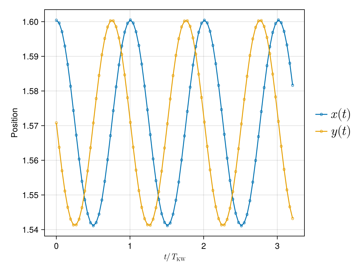

We see that the $x$ and $y$ positions of the chosen point oscillate sinusoidally. The period of the oscillations are very close to the expected Kelvin wave period $T_{\text{KW}}$.

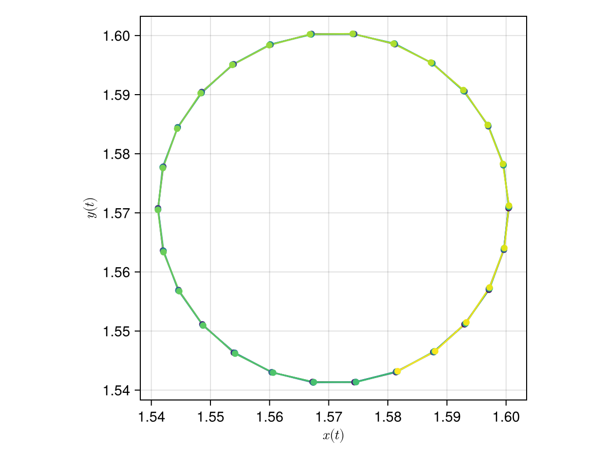
The oscillations above suggest circular trajectories, as we can check in the following figure:

scatterlines(
    xpos, ypos;
    color = tnorm,
    axis = (aspect = DataAspect(), xlabel = L"x(t)", ylabel = L"y(t)"),
)

Measuring performance

The VortexPasta solver uses the TimerOutputs.jl package to estimate the time spent (and memory allocated) in different stages of the computation.

Accessing timing information is very simple, as it is all included in the to field of the VortexFilamentSolver:

iter.to

──────────────────────────────────────────────────────────────────────────────────────────────────────
                                                             Time                    Allocations
                                                    ───────────────────────   ────────────────────────
                 Tot / % measured:                       17.0s /  39.6%           1.36GiB /  21.5%

Section                                     ncalls     time    %tot     avg     alloc    %tot      avg
──────────────────────────────────────────────────────────────────────────────────────────────────────
Update values at nodes                       10.9k    4.90s   72.8%   450μs    219MiB   72.9%  20.6KiB
  Biot-Savart (LIA only)                     10.6k    3.00s   44.6%   282μs    127MiB   42.2%  12.2KiB
    Add point charges                        10.6k    1.74s   25.9%   164μs   45.2MiB   15.0%  4.35KiB
    Short-range component (async)            10.6k    1.02s   15.2%  96.4μs   52.6MiB   17.5%  5.07KiB
      Local term (LIA)                       10.6k    937ms   13.9%  88.2μs   22.7MiB    7.5%  2.19KiB
      Copy point charges (host -> device)    10.6k   46.1ms    0.7%  4.34μs   16.9MiB    5.6%  1.62KiB
      Synchronise GPU                        10.6k    396μs    0.0%  37.3ns     0.00B    0.0%    0.00B
    Copy output (device -> host)             10.6k   24.7ms    0.4%  2.33μs   2.43MiB    0.8%     240B
    Wait for async task to finish            10.6k   2.36ms    0.0%   222ns     0.00B    0.0%    0.00B
  Biot-Savart (excluding LIA)                  166    871ms   13.0%  5.25ms   23.5MiB    7.8%   145KiB
    Long-range component (async)               166    495ms    7.4%  2.98ms   14.7MiB    4.9%  90.5KiB
      Vorticity to Fourier                     166    268ms    4.0%  1.61ms   7.44MiB    2.5%  45.9KiB
      Interpolate to physical                  166    202ms    3.0%  1.22ms   6.00MiB    2.0%  37.0KiB
      Velocity field (Fourier)                 166   22.1ms    0.3%   133μs    573KiB    0.2%  3.45KiB
      Copy point charges (host -> device)      166   1.29ms    0.0%  7.79μs    319KiB    0.1%  1.92KiB
      Process point charges                    166    175μs    0.0%  1.05μs     0.00B    0.0%    0.00B
      Synchronise GPU                          166   6.11μs    0.0%  36.8ns     0.00B    0.0%    0.00B
    Short-range component (async)              166    163ms    2.4%   982μs   2.03MiB    0.7%  12.5KiB
      Pair interactions                        166    132ms    2.0%   795μs    416KiB    0.1%  2.51KiB
      Remove self-interactions                 166   21.5ms    0.3%   129μs    397KiB    0.1%  2.39KiB
      Process point charges                    166   6.54ms    0.1%  39.4μs    605KiB    0.2%  3.64KiB
      Copy point charges (host -> device)      166   1.80ms    0.0%  10.8μs    353KiB    0.1%  2.12KiB
      Synchronise GPU                          166   6.45μs    0.0%  38.9ns     0.00B    0.0%    0.00B
    Add point charges                          166   25.9ms    0.4%   156μs    724KiB    0.2%  4.36KiB
    Copy output (device -> host)               332   1.26ms    0.0%  3.81μs    127KiB    0.0%     392B
    Wait for async task to finish              332   85.3μs    0.0%   257ns     0.00B    0.0%    0.00B
    CPU-only operations (synchronous)          166   14.0μs    0.0%  84.5ns     0.00B    0.0%    0.00B
  Biot-Savart (full)                            83    482ms    7.2%  5.81ms   13.0MiB    4.3%   160KiB
    Long-range component (async)                83    367ms    5.5%  4.42ms   10.6MiB    3.5%   131KiB
      Interpolate to physical                  166    207ms    3.1%  1.25ms   5.99MiB    2.0%  37.0KiB
      Vorticity to Fourier                      83    138ms    2.1%  1.66ms   3.72MiB    1.2%  45.9KiB
      Velocity field (Fourier)                  83   11.3ms    0.2%   136μs    287KiB    0.1%  3.45KiB
      Streamfunction field (Fourier)            83   9.64ms    0.1%   116μs    287KiB    0.1%  3.45KiB
      Copy point charges (host -> device)       83    593μs    0.0%  7.15μs    160KiB    0.1%  1.92KiB
      Process point charges                     83   95.4μs    0.0%  1.15μs     0.00B    0.0%    0.00B
      Synchronise GPU                           83   3.05μs    0.0%  36.8ns     0.00B    0.0%    0.00B
    Short-range component (async)               83   93.4ms    1.4%  1.13ms   1.38MiB    0.5%  17.1KiB
      Pair interactions                         83   67.4ms    1.0%   812μs    220KiB    0.1%  2.66KiB
      Remove self-interactions                  83   11.2ms    0.2%   135μs    214KiB    0.1%  2.58KiB
      Local term (LIA)                          83   9.65ms    0.1%   116μs    187KiB    0.1%  2.25KiB
      Process point charges                     83   2.98ms    0.0%  35.9μs    301KiB    0.1%  3.62KiB
      Copy point charges (host -> device)      166   1.32ms    0.0%  7.97μs    311KiB    0.1%  1.88KiB
      Synchronise GPU                           83   3.02μs    0.0%  36.4ns     0.00B    0.0%    0.00B
    Add point charges                           83   18.0ms    0.3%   217μs    361KiB    0.1%  4.34KiB
    Copy output (device -> host)               166    870μs    0.0%  5.24μs   77.5KiB    0.0%     478B
    CPU-only operations (synchronous)           83   74.8μs    0.0%   901ns     0.00B    0.0%    0.00B
    Wait for async task to finish              166   51.1μs    0.0%   308ns     0.00B    0.0%    0.00B
Advect filaments                             10.9k    1.68s   25.1%   155μs   70.9MiB   23.6%  6.68KiB
Callback                                        83    118ms    1.8%  1.42ms   8.48MiB    2.8%   105KiB
After advection                                 83   17.3ms    0.3%   208μs    388KiB    0.1%  4.68KiB
  Fold and refine                               83   16.5ms    0.2%   199μs    373KiB    0.1%  4.50KiB
  Reconnect                                     83    202μs    0.0%  2.43μs   6.48KiB    0.0%    80.0B
Prepare interpolable fields                     83   8.95ms    0.1%   108μs   1.78MiB    0.6%  21.9KiB
Resize timestepping cache                       83    183μs    0.0%  2.21μs     0.00B    0.0%    0.00B
──────────────────────────────────────────────────────────────────────────────────────────────────────

We can see that, in this particular case, the runtime is mostly dominated by the the LIA (local) term, which is computed much more often than the non-local interactions due to the use of a splitting scheme for the temporal evolution.

Fourier analysis

Spatial analysis

The idea is to identify the spatial fluctuations of a single vortex with respect to the unperturbed filament. For this, we first write the perturbations in complex representation as a function of the $z$ coordinate, i.e. $w(z)=x(z)+iy(z)$.

We want to apply the FFT to these two functions. For this, we need all points of the vortex filament to be equispaced in $z$:

f = iter.fs[1]               # vortex to analyse
zs = [s⃗.z for s⃗ in f]  # y locations
N = length(zs)
zs_expected = range(zs[begin], zs[begin] + L; length = N + 1)[1:N]  # equispaced locations
isapprox(zs, zs_expected; rtol = 1e-5)  # check that z locations are approximately equispaced

true

Now that we have verified this, we define the complex function $w(z)=x(z)+iy(z)$ and we perform a complex-to-complex FFT to obtain $\hat{w}(k)$:

xs = [s⃗.x for s⃗ in f]  # x locations
ys = [s⃗.y for s⃗ in f]  # y locations
ws = @. xs + im * ys

using FFTW: fft, fft!, fftfreq, fftshift
w_hat = fft(ws)
@. w_hat = w_hat / N  # normalise FFT
@show w_hat[1]       # the zero frequency gives the mean location
w_hat[1] ≈ π/2 + π/2 * im  # we expect the mean location to be (π/2, π/2)

true

The associated wavenumbers are multiples of $2\pi /\Delta z=2\pi N/L$:

Δz = L / N
@assert isapprox(Δz, zs[2] - zs[1]; rtol = 1e-4)
ks = fftfreq(N, 2π / Δz)
ks'  # should be integers if L = 2π

1×64 adjoint(::AbstractFFTs.Frequencies{Float64}) with eltype Float64:
 0.0  1.0  2.0  3.0  4.0  5.0  6.0  …  -6.0  -5.0  -4.0  -3.0  -2.0  -1.0

Note that this includes positive and negative wavenumbers. More precisely, ks[2:N÷2] contains the positive wavenumbers, and ks[N÷2+1:end] contains the corresponding negative wavenumbers.

We now want to compute the wave action spectrum $n(k)=|\hat{w}(k){|}^2+|\hat{w}(-k){|}^2$, which is related to the amplitude of the oscillations at the scale $\lambda =2\pi /k$.

function wave_action_spectrum(ks::AbstractVector, w_hat::AbstractVector)
    @assert ks[2] == -ks[end]  # contains positive and negative wavenumbers
    @assert length(ks) == length(w_hat)
    N = length(ks)
    dk = ks[2]  # this is the wavenumber increment
    if iseven(N)
        Nh = N ÷ 2
        @assert ks[Nh + 1] ≈ -(ks[Nh] + dk)  # wavenumbers change sign after index Nh
    else
        Nh = N ÷ 2 + 1
        @assert ks[Nh + 1] == -ks[Nh]  # wavenumbers change sign after index Nh
    end
    ks_pos = ks[2:Nh]  # only positive wavenumbers
    nk = similar(ks_pos)
    for j ∈ eachindex(ks_pos)
        local k = ks_pos[j]
        i⁺ = 1 + j      # index of coefficient corresponding to wavenumber +k
        i⁻ = N + 1 - j  # index of coefficient corresponding to wavenumber -k
        @assert ks[i⁺] == -ks[i⁻] == k  # verification
        nk[j] = abs2(w_hat[i⁺]) + abs2(w_hat[i⁻])
    end
    ks_pos, nk
end

ks_pos, nk = wave_action_spectrum(ks, w_hat)
nk_normalised = nk ./ ((ϵ * L)^2 / 2)
sum(nk_normalised)  # we expect the sum to be 1

0.9999943963069883

We can finally plot the final state:

fig = Figure()
ax = Axis(
    fig[1, 1];
    xscale = log10, yscale = log10, xlabel = L"k", ylabel = L"2 \, n(k) / (ϵ L)^2",
    xlabelsize = 20, ylabelsize = 20,
    xticks = LogTicks(0:4), xminorticksvisible = true, xminorticks = IntervalsBetween(9),
    yminorticksvisible = true, yminorticks = exp10.(-40:10),
)
scatterlines!(ax, ks_pos, nk_normalised)
xlims!(ax, 0.8 * ks_pos[begin], nothing)
ylims!(ax, 1e-30, 1e1)
vlines!(ax, ks_pos[m]; linestyle = :dash, color = :orangered)
fig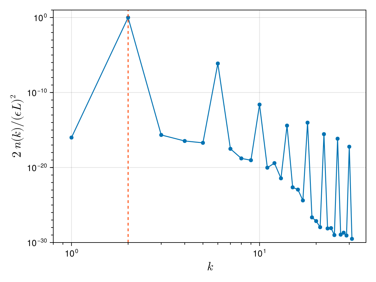

We see that the wave action spectrum is strongly peaked at the wavenumber $k=2\pi m/L$ (dashed vertical line) corresponding to the perturbation mode $m$ we chose at the beginning. Note that the other peaks (which here are about 6 orders of magnitude smaller than the main peak) are not numerical artefacts. Instead, these peaks appearing at wavenumbers $q=k(1+2n)$ for integer $n$ can be explained analytically (see box below). Their relative magnitude should further decrease if one decreases the perturbation amplitude.

A kind of proof using LIA

One way to illustrate this analytically is using the local induction approximation (LIA). Let's consider the perturbed line $\mathit{s}(z)=[ϵ\sin (z),0,z]$ parametrised by the $z$ coordinate. The LIA can be written as

$${\mathit{v}}_{\text{LIA}}=C\frac{{\mathit{s}}^{\prime }\times {\mathit{s}}^{″}}{|{\mathit{s}}^{\prime }{|}^3}$$

where $C$ is (roughly) a constant. Derivatives are with respect to the chosen parametrisation (which can differ from the "natural" arc-length parametrisation), hence the normalising factor in the denominator.

In our case we have ${\mathit{s}}^{\prime }=[ϵ\cos (z),0,1]$ and ${\mathit{s}}^{″}=[-ϵ\sin (z),0,0]$, and thus

$$v_{\text{LIA}}=\frac{Cϵ\sin (z)}{(1+{ϵ}^2{\cos }^{2}z{)}^{3/2}}.$$

Using a Taylor expansion, one can easily show that the denominator introduces fluctuations over the odd harmonics $q=1+2n$ for $n\in \{1,2,3,\dots \}$:

$$v_{\text{LIA}}=Cϵ\sin (z)[1-\frac{3}{2}{ϵ}^2{\cos }^{2}z+\mathcal{O}({ϵ}^4)].$$

Noting that $\sin (z){\cos }^2(z)=[\sin (z)+\sin (3z)]/4$, one clearly sees that the term in ${ϵ}^2$ excites modes at wavenumber $q=3$, i.e. the third harmonic of the perturbed mode $k=1$. Since the contribution is proportional to ${ϵ}^2$, this non-linear effect should be negligible for very small perturbation amplitudes. It is easy to see that all of this generalises to all odd harmonics $q=1+2n$ by taking into account higher-order terms of the Taylor expansion.

In the tutorial, we initially perturbed the mode $k=2$, which excites its odd harmonics $q=k(1+2n)=6,10,14,\dots$ as seen in the above figure.

We also see that the sum ${\sum }_{k}n(k)$ (which is basically just the value of the main peak in this case) is equal to $A^2/2$, where $A=ϵL$ is the amplitude of the initial perturbation.

The main conclusion is that, when we perturb a single Kelvin wave mode as we did here, that original mode is exactly preserved over time (except for negligible high-order effects).

Temporal analysis

We can do something similar to analyse the temporal oscillations of the filament. For example, we can take the same temporal data we analysed before, corresponding to the position of a single filament node:

xt = getindex.(X_probe, 1)  # x positions of a single node over time
yt = getindex.(X_probe, 2)  # y positions of a single node over time
zt = getindex.(X_probe, 3)  # z positions of a single node over time
std(zt) / mean(zt)    # ideally, the z positions shouldn't change over time

1.66220572399868e-5

Similarly to before, we now write $w(t)=x(t)+iy(t)$ and perform an FFT:

inds_t = eachindex(times)[begin:end - 1]  # don't consider the last time to make sure the timestep Δt is constant
w_equilibrium = 0.25L + im * 0.25L  # equilibrium position of first vortex (w = x + iy)
wt = @views @. xt[inds_t] + im * yt[inds_t] - w_equilibrium  # we subtract the equilibrium position
Nt = length(wt)           # number of time snapshots
Δt = times[2] - times[1]  # timestep
@assert times[begin:end-1] ≈ range(times[begin], times[end-1]; length = Nt)  # check that times are equispaced
w_hat = fft(wt)
@. w_hat = w_hat / Nt  # normalise FFT
ωs = fftfreq(Nt, 2π / Δt)

ωs_pos, nω = wave_action_spectrum(ωs, w_hat)
ωs_normalised = ωs_pos ./ ω_kw  # normalise by expected KW frequency

fig = Figure()
ax = Axis(
    fig[1, 1];
    xscale = log10, yscale = log10, xlabel = L"ω / ω_{\text{kw}}", ylabel = L"n(ω)",
    xlabelsize = 20, ylabelsize = 20,
    xticks = LogTicks(0:4), xminorticksvisible = true, xminorticks = IntervalsBetween(9),
    yticks = LogTicks(-20:10), yminorticksvisible = true, yminorticks = IntervalsBetween(9),
)
scatterlines!(ax, ωs_normalised, nω; label = "Original signal")
xlims!(ax, 0.8 * ωs_normalised[begin], 1.2 * ωs_normalised[end])
vlines!(ax, 1.0; linestyle = :dash, color = :orangered)
fig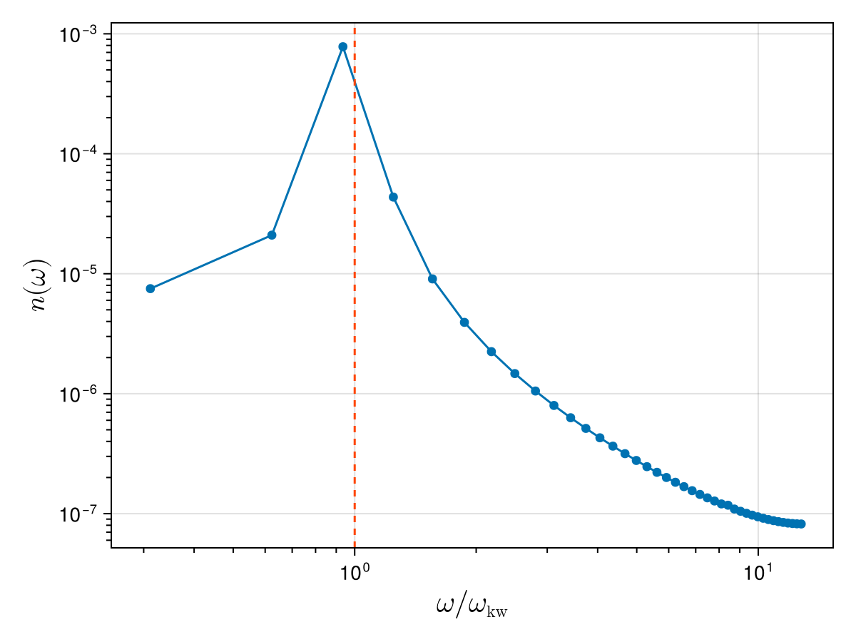

We see that the temporal spectrum is strongly peaked near the analytical Kelvin wave frequency (dashed vertical line). However, since the trajectory is not perfectly periodic in time (the signal is discontinuous when going from the final time to the initial time), other frequencies are also present in the spectrum (this is known as spectral leakage).

To reduce the effect of spectral leakage, the usual solution is to apply a window function to the original signal to make it periodic. There are many examples of window functions which are commonly used in signal processing.

Here we use the DSP.jl package which includes many definitions of window functions. Note that we first need to subtract the mean value from our input signal before multiplying it by the window function. Below we compare the previous temporal spectrum with the one obtained after applying the Hann window:

using DSP: DSP

wt_mean = mean(wt)
window = DSP.Windows.hanning(Nt)
wt_windowed = @. (wt - wt_mean) * window
w_hat = fft(wt_windowed)
@. w_hat = w_hat / Nt  # normalise FFT
_, nω_windowed = wave_action_spectrum(ωs, w_hat)

scatterlines!(ax, ωs_normalised, nω_windowed; label = "Windowed signal")
Legend(fig[0, 1], ax; orientation = :horizontal, framevisible = false, colgap = 32, patchsize = (40, 10))
rowgap!(fig[:, 1].layout, 6)  # reduce gap between plot and legend (default gap is 18)
fig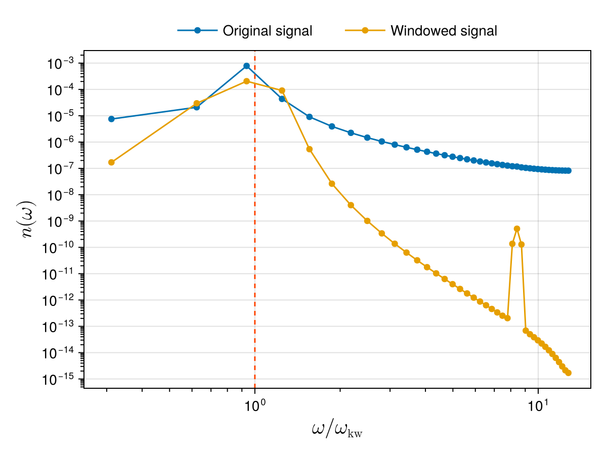

The new spectrum is still peaked near the expected frequency, while artificial modes far from this frequency are strongly damped compared to the original spectrum. Note however that windowing tends to smoothen the spectrum around the analytical Kelvin wave frequency.

Dispersion relation

To verify the dispersion relation of Kelvin waves, we perform a new simulation where we initially excite a large range of wavenumbers $k$, instead of just perturbing a single scale as above.

Creating the initial condition

We start by defining one straight filament:

p = PeriodicLine()  # no perturbation, we will perturb it afterwards
w_equilibrium = 0.25L + im * 0.25L  # equilibrium position of vortex (w = x + iy)
S = define_curve(p; scale = (+L, +L, +L), translate = (0.25L, 0.25L, 0.5L))
f = Filaments.init(S, ClosedFilament, N, QuinticSplineMethod())

We then perturb each point of the filament with random translations in the $x$ and $y$ directions. We define the perturbation in Fourier space, which allows to select the range of wavenumbers $k$ which will be perturbed.

using FFTW: fft, bfft, fftfreq

w_hat = zeros(ComplexF64, N)  # perturbation in Fourier space
ks = fftfreq(N, 2π * N / L)   # wavenumbers associated to perturbation, in [-N/2, +N/2-1]
kmax = π * N / L
kmax_perturb = 0.5 * kmax   # perturb up to this wavenumber (to avoid issues at the discretisation scale)
A_rms = 1e-6 * L  # perturbation amplitude (wanted rms value of ws[:])

using StableRNGs: StableRNG  # for deterministic random number generation
rng = StableRNG(42)  # initialise random number generator (RNG)

for i in eachindex(w_hat, ks)
    kabs = abs(ks[i])
    if 0 < kabs <= kmax_perturb
        w_hat[i] = randn(rng, ComplexF64)  # perturb all wavenumbers equally
    else
        w_hat[i] = 0
    end
end
factor = A_rms / sqrt(sum(abs2, w_hat))
w_hat .*= factor

Now convert to physical space and update filament points:

ws = bfft(w_hat)  # inverse FFT
for i in eachindex(f, ws)
    w = ws[i]
    f[i] += Vec3(real(w), imag(w), 0)
end
update_coefficients!(f)

Finally, create the other vortices by mirror symmetry.

# Helper function which creates a new filament by mirror symmetry with respect to a given plane.
function create_mirror(f::AbstractFilament; xplane = nothing, yplane = nothing, zplane = nothing)
    planes = (xplane, yplane, zplane)
    nplanes = sum(!isnothing, planes)
    nplanes == 1 || error("expected exactly a single symmetry plane")
    g = Filaments.similar_filament(f; offset = -end_to_end_offset(f))  # opposite end-to-end offset
    for i in eachindex(f, g)
        j = lastindex(f) + 1 - i  # we switch the orientation of the filament
        g[i] = map(f[j], planes) do x, xmid
            xmid === nothing ? x : (2 * xmid - x)
        end
    end
    update_coefficients!(g)
    g
end

fx = create_mirror(f; xplane = L/2)  # mirror symmetry wrt x = L/2 plane
fy = create_mirror(f; yplane = L/2)  # mirror symmetry wrt y = L/2 plane
fxy = create_mirror(fx; yplane = L/2)  # mirror symmetry of fx wrt y = L/2 plane

fs = [f, fx, fy, fxy]

plot_filaments(fs)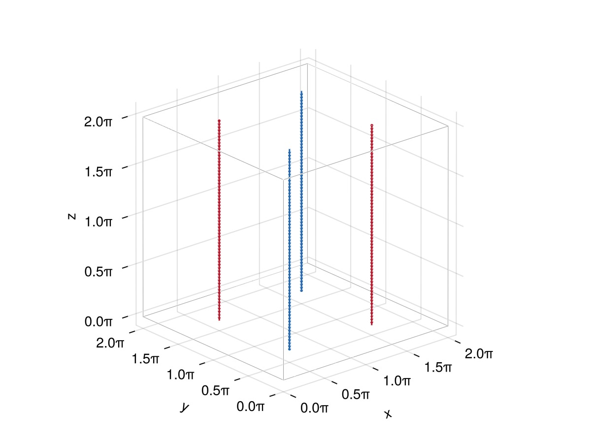

We can now take a look at the wave action spectrum associated to this initial condition to check that, this time, the excited wavenumbers have roughly the same amplitudes:

xs = [s⃗.x for s⃗ in f]  # x locations
ys = [s⃗.y for s⃗ in f]  # y locations
ws = @. xs + im * ys
w_hat = fft(ws) ./ N  # normalised FFT

ks_pos, nk = wave_action_spectrum(ks, w_hat)
nk_normalised = nk ./ A_rms^2

fig = Figure()
ax = Axis(
    fig[1, 1];
    xscale = log10, yscale = log10, xlabel = L"k", ylabel = L"n(k) / A_{\text{rms}}^2",
    xlabelsize = 20, ylabelsize = 20,
    xticks = LogTicks(0:4), xminorticksvisible = true, xminorticks = IntervalsBetween(9),
    yminorticksvisible = true, yminorticks = exp10.(-40:10),
)
scatterlines!(ax, ks_pos, nk_normalised)
xlims!(ax, 0.8 * ks_pos[begin], nothing)
fig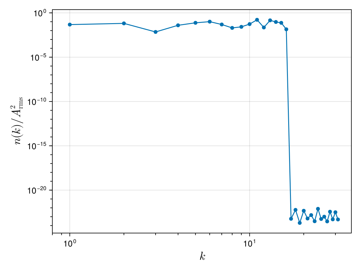

Running the simulation

We create a new problem with this initial condition and with the same parameters as before (except for a longer simulation time):

Tsim = kelvin_wave_period(L; a, Δ, Γ)
prob = VortexFilamentProblem(fs, Tsim, params)

VortexFilamentProblem with fields:
 ├─ p: ParamsBiotSavart{Float64}(Γ = 1.0, a = 1.0e-8, Δ = 0.25, α = 1.4285714285714286, …)
 ├─ tspan: (0.0, 4.202824549610985) -- simulation timespan
 └─ fs: 4-element VectorOfVectors -- vortex filaments at t = 0.0

We want to store the whole history of complex positions $w(z,t)$ of the locations of the nodes of a single filament. We store this in a vector, and we reshape it after the simulation:

const ws_vec = ComplexF64[]

function callback_random(iter)
    (; nstep, t,) = iter
    if nstep == 0  # make sure vectors are empty at the beginning of the simulation
        empty!(times)
        empty!(energy)
        empty!(ws_vec)
    end
    E = Diagnostics.kinetic_energy(iter)
    push!(times, t)
    push!(energy, E)
    # Save locations of the first filament in complex form
    for s⃗ in iter.fs[1]
        w = s⃗.x + im * s⃗.y
        push!(ws_vec, w)
    end
    nothing
end

δ = minimum_node_distance(prob.fs)  # should be close to L/N in our case
dt_kw = kelvin_wave_period(δ; a, Δ, Γ)
scheme = Strang(RK4(); nsubsteps = 2)
dt = 2 * scheme.nsubsteps * dt_kw

iter = init(prob, scheme; dt, callback = callback_random, fast_term = LocalTerm())
reset_timer!(iter.to)  # to get more accurate timings (removes most of the compilation time)
solve!(iter)
iter.to

────────────────────────────────────────────────────────────────────────────────
                                       Time                    Allocations      
                              ───────────────────────   ────────────────────────
      Tot / % measured:            19.5s /  93.9%            807MiB /  80.9%    

Section               ncalls     time    %tot     avg     alloc    %tot      avg
────────────────────────────────────────────────────────────────────────────────
Update values at n...  15.2k    15.6s   85.1%  1.03ms    528MiB   80.9%  35.7KiB
  Biot-Savart (exc...  1.60k    6.65s   36.2%  4.16ms    179MiB   27.3%   115KiB
    Long-range com...  1.60k    4.76s   26.0%  2.98ms    141MiB   21.6%  90.4KiB
      Vorticity to...  1.60k    2.57s   14.0%  1.61ms   71.5MiB   10.9%  45.8KiB
      Interpolate ...  1.60k    1.96s   10.7%  1.23ms   57.6MiB    8.8%  37.0KiB
      Velocity fie...  1.60k    200ms    1.1%   125μs   5.38MiB    0.8%  3.45KiB
      Copy point c...  1.60k   11.8ms    0.1%  7.42μs   3.00MiB    0.5%  1.92KiB
      Process poin...  1.60k   1.31ms    0.0%   818ns     0.00B    0.0%    0.00B
      Synchronise GPU  1.60k   60.5μs    0.0%  37.9ns     0.00B    0.0%    0.00B
    Short-range co...  1.60k    1.56s    8.5%   975μs   19.5MiB    3.0%  12.5KiB
      Pair interac...  1.60k    1.26s    6.9%   791μs   3.89MiB    0.6%  2.50KiB
      Remove self-...  1.60k    209ms    1.1%   131μs   3.79MiB    0.6%  2.43KiB
      Process poin...  1.60k   60.5ms    0.3%  37.9μs   5.65MiB    0.9%  3.62KiB
      Copy point c...  1.60k   14.3ms    0.1%  8.93μs   3.31MiB    0.5%  2.12KiB
      Synchronise GPU  1.60k   61.7μs    0.0%  38.7ns     0.00B    0.0%    0.00B
    Add point charges  1.60k    285ms    1.6%   179μs   6.79MiB    1.0%  4.36KiB
    Copy output (d...  3.19k   10.0ms    0.1%  3.13μs   1.11MiB    0.2%     363B
    Wait for async...  3.19k    773μs    0.0%   242ns     0.00B    0.0%    0.00B
    CPU-only opera...  1.60k   94.8μs    0.0%  59.4ns     0.00B    0.0%    0.00B
  Biot-Savart (full)     798    4.62s   25.2%  5.79ms    125MiB   19.1%   160KiB
    Long-range com...    798    3.50s   19.1%  4.39ms    102MiB   15.7%   131KiB
      Interpolate ...  1.60k    2.00s   10.9%  1.25ms   57.7MiB    8.8%  37.0KiB
      Vorticity to...    798    1.28s    7.0%  1.61ms   35.7MiB    5.5%  45.9KiB
      Velocity fie...    798    116ms    0.6%   145μs   2.71MiB    0.4%  3.48KiB
      Streamfuncti...    798   87.6ms    0.5%   110μs   2.69MiB    0.4%  3.45KiB
      Copy point c...    798   5.99ms    0.0%  7.51μs   1.50MiB    0.2%  1.92KiB
      Process poin...    798    715μs    0.0%   896ns     0.00B    0.0%    0.00B
      Synchronise GPU    798   30.2μs    0.0%  37.9ns     0.00B    0.0%    0.00B
    Short-range co...    798    925ms    5.0%  1.16ms   13.3MiB    2.0%  17.0KiB
      Pair interac...    798    675ms    3.7%   846μs   2.09MiB    0.3%  2.68KiB
      Remove self-...    798    109ms    0.6%   137μs   1.99MiB    0.3%  2.56KiB
      Local term (...    798   95.3ms    0.5%   119μs   1.75MiB    0.3%  2.25KiB
      Process poin...    798   27.8ms    0.2%  34.9μs   2.83MiB    0.4%  3.64KiB
      Copy point c...  1.60k   11.1ms    0.1%  6.98μs   2.92MiB    0.4%  1.88KiB
      Synchronise GPU    798   29.7μs    0.0%  37.2ns     0.00B    0.0%    0.00B
    Add point charges    798    167ms    0.9%   209μs   3.39MiB    0.5%  4.35KiB
    Copy output (d...  1.60k   7.10ms    0.0%  4.45μs    647KiB    0.1%     415B
    CPU-only opera...    798    625μs    0.0%   783ns     0.00B    0.0%    0.00B
    Wait for async...  1.60k    460μs    0.0%   288ns     0.00B    0.0%    0.00B
  Biot-Savart (LIA...  12.8k    3.97s   21.6%   311μs    154MiB   23.6%  12.4KiB
    Add point charges  12.8k    2.57s   14.0%   201μs   59.4MiB    9.1%  4.77KiB
    Short-range co...  12.8k    1.24s    6.8%  97.5μs   63.3MiB    9.7%  5.07KiB
      Local term (...  12.8k    1.13s    6.2%  88.8μs   27.3MiB    4.2%  2.19KiB
      Copy point c...  12.8k   59.5ms    0.3%  4.66μs   20.3MiB    3.1%  1.62KiB
      Synchronise GPU  12.8k    481μs    0.0%  37.7ns     0.00B    0.0%    0.00B
    Copy output (d...  12.8k   29.4ms    0.2%  2.30μs   2.93MiB    0.4%     240B
    Wait for async...  12.8k   3.00ms    0.0%   235ns     0.00B    0.0%    0.00B
Advect filaments       15.2k    2.37s   12.9%   156μs   98.8MiB   15.1%  6.67KiB
After advection          798    182ms    1.0%   228μs   3.60MiB    0.6%  4.62KiB
  Fold and refine        798    176ms    1.0%   221μs   3.47MiB    0.5%  4.45KiB
  Reconnect              798   1.49ms    0.0%  1.86μs   62.3KiB    0.0%    80.0B
Prepare interpolab...    798    113ms    0.6%   141μs   17.1MiB    2.6%  21.9KiB
Callback                 798   73.5ms    0.4%  92.1μs   5.57MiB    0.9%  7.14KiB
Resize timesteppin...    798   1.46ms    0.0%  1.83μs     0.00B    0.0%    0.00B
────────────────────────────────────────────────────────────────────────────────

Once again, kinetic energy is quite well conserved:

std(energy) / mean(energy)

2.7857064677441644e-11

In fact energy slightly decreases:

(energy[end] - energy[begin]) / energy[begin]

-9.516637443734871e-11

which can be explained by numerical dissipation at the smallest resolved scales. Notice that the spectrum gets populated at large wavenumbers, which is possibly due to the Kelvin wave cascade mechanism:

ws_mat = reshape(ws_vec, N, :)  # reinterpret 1D vector as a 2D matrix: ws_mat[i, j] = w(z_i, t_j)
@views _, nk_start = wave_action_spectrum(ks, fft(ws_mat[:, begin]) ./ N)
@views _, nk_end = wave_action_spectrum(ks, fft(ws_mat[:, end]) ./ N)
fig = Figure()
ax = Axis(
    fig[1, 1];
    xscale = log10, yscale = log10, xlabel = L"k", ylabel = L"n(k) / A_{\text{rms}}^2",
    xlabelsize = 20, ylabelsize = 20,
    xticks = LogTicks(0:4), xminorticksvisible = true, xminorticks = IntervalsBetween(9),
    yminorticksvisible = true, yminorticks = exp10.(-40:10),
)
scatterlines!(ax, ks_pos, nk_start ./ A_rms^2; label = "Initial time")
scatterlines!(ax, ks_pos, nk_end ./ A_rms^2; label = "Final time")
xlims!(ax, 0.8 * ks_pos[begin], nothing)
axislegend(ax; position = (0, 0))
fig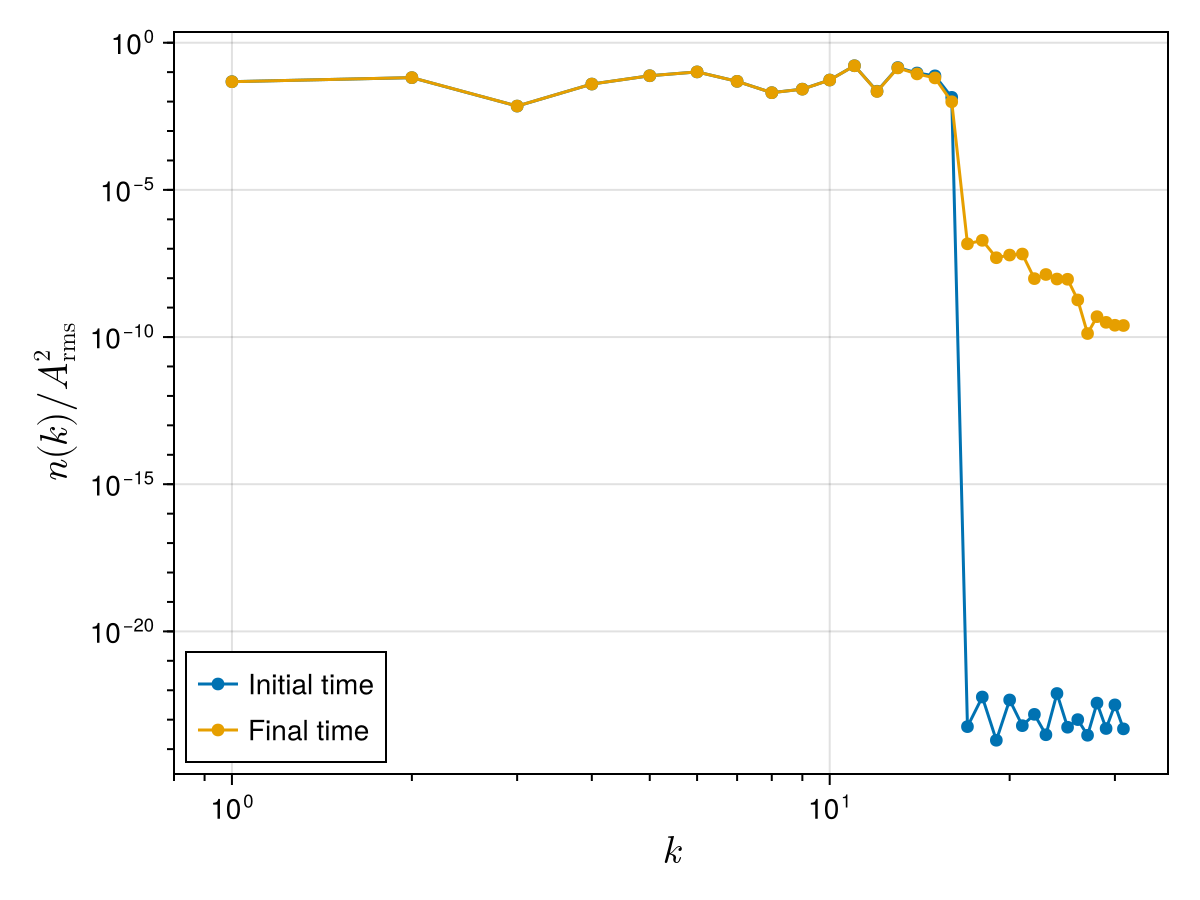

Verifying the Kelvin wave dispersion relation

We will assume that the simulation is in a statistically stationary state, which allows to perform FFTs in time as well as in space.

We start by choosing the times over which we will analyse the data. Currently we analyse all times, but this could be modified in simulations which require some time before reaching a (near-)stationary state.

t_inds = eachindex(times)[begin:end]  # this may be modified to use a subset of the simulation time
Nt = length(t_inds)   # number of timesteps to analyse
ws_h = ws_mat[:, t_inds]  # create copy of positions to avoid modifying the simulation output
ws_h .-= w_equilibrium    # subtract equilibrium position

64×799 Matrix{ComplexF64}:
 -4.15535e-6+4.64122e-6im  …   -4.2791e-6-1.88914e-6im
  1.32043e-6+6.59221e-6im     -4.93763e-6+5.3689e-6im
   4.9057e-6+7.76414e-6im     -4.19102e-6+8.46733e-6im
  1.56307e-6+5.96558e-6im     -9.88867e-7+3.89358e-6im
 -3.99974e-6+2.7909e-7im       2.98489e-6-4.45523e-7im
 -3.74592e-6-4.66318e-6im  …   3.59489e-6+1.30238e-6im
  1.58423e-6-3.24128e-6im     -7.28623e-7+4.95071e-6im
  3.31877e-6+2.73898e-6im     -6.27256e-6+4.86334e-6im
 -1.82543e-6+6.06245e-6im     -7.55109e-6+1.78905e-6im
 -6.59718e-6+4.32956e-6im     -2.79821e-6-1.28419e-6im
            ⋮              ⋱  
 -1.12477e-5+3.80923e-6im  …  -9.32702e-6-2.19986e-6im
 -3.64297e-6-4.16605e-6im      -2.2791e-6+2.61882e-6im
  4.25811e-6-7.93425e-6im      3.13886e-6+4.94948e-6im
   4.3955e-6-3.3357e-6im       1.52284e-6+1.07325e-6im
  5.70624e-7+3.45148e-6im     -2.11861e-6-2.59298e-6im
 -4.09761e-7+5.23592e-6im  …  -2.58823e-6+1.51288e-7im
  6.03639e-7+2.68405e-6im     -1.33013e-6+4.35545e-6im
 -1.14974e-6+1.09316e-6im     -1.52195e-6+2.15169e-6im
 -4.68204e-6+2.39272e-6im     -2.99737e-6-3.12112e-6im

As detailed in the Temporal analysis section, we apply a window function over the temporal dimension since the original signal is not exactly periodic in time:

window = DSP.Windows.hanning(Nt)
for i ∈ axes(ws_h, 1)
    @. @views ws_h[i, :] *= window
end

We can now perform a 2D FFT and plot the results:

fft!(ws_h)  # in-place FFT
ws_h ./= length(ws_h)  # normalise FFT

# Combine +k and -k wavenumbers and plot as a function of |k| (results should be symmetric anyways)
ws_abs2 = @views abs2.(ws_h[1:((end + 1)÷2), :])  # from k = 0 to k = +kmax
@views ws_abs2[2:end, :] .+= abs2.(ws_h[end:-1:(end÷2 + 2), :])  # from -kmax to -1

Δt = times[2] - times[1]  # timestep
ks_pos = ks[1:(end + 1)÷2]  # wavenumbers (≥ 0 only)
ωs = fftfreq(Nt, 2π / Δt)     # frequencies
ωs_shift = fftshift(ωs)   # for visualisation: make sure ω is in increasing order
w_plot = fftshift(log10.(ws_abs2), (2,))  # FFT shift along second dimension (frequencies)

k_max = ks_pos[end]       # maximum wavenumber
ω_max = -ωs_shift[begin]  # maximum frequency

# Analytical dispersion relation
ks_fine = range(0, k_max; step = ks_pos[2] / 4)
ωs_kw = @. -Γ * ks_fine^2 / (4 * π) * (
    log(2 / (abs(ks_fine) * a)) - γ + 1/2 - Δ
)

# We also plot the wavenumber associated to the mean inter-vortex distance for reference
ℓ = sqrt(params.Ls[1] * params.Ls[2] / length(fs))  # mean inter-vortex distance
k_ℓ = 2π / ℓ

fig = Figure()
ax = Axis(fig[1, 1]; xlabel = L"k", ylabel = L"ω")
xlims!(ax, 0.8 * k_max .* (0, 1))
ylims!(ax, 0.8 * ω_max .* (-1, 1))
hm = heatmap!(
    ax, ks_pos, ωs_shift, w_plot;
    colormap = Reverse(:deep),
    colorrange = round.(Int, extrema(w_plot)) .+ (4, 0),
)
Colorbar(fig[1, 2], hm; label = L"\log \, |\hat{w}|^2", labelsize = 20)
hlines!(ax, 0; color = :white, linestyle = :dash, linewidth = 1)
let color = :lightblue
    vlines!(ax, k_ℓ; color, linestyle = :dot)
    text!(ax, L"\frac{2π}{ℓ}"; position = (k_ℓ, -0.8 * ω_max), offset = (6, 4), align = (:left, :bottom), color, fontsize = 16)
end
lines!(ax, ks_fine, ωs_kw; color = (:orangered, 1.0), linestyle = :dash, linewidth = 1)
fig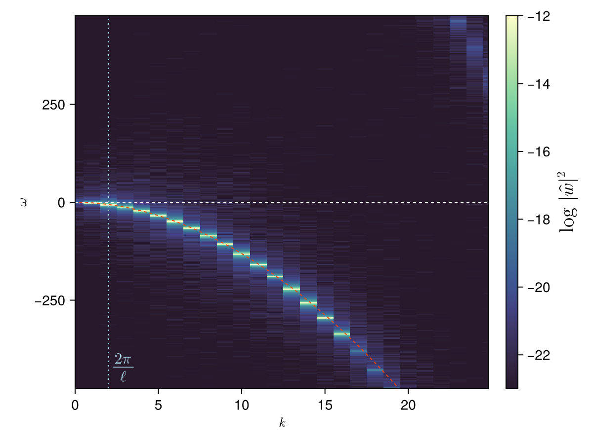

Fluctuations are clearly concentrated on the analytical dispersion relation ${\omega }_{\text{KW}}(k)$ given at the beginning of the tutorial (orange dashed line).

---

This page was generated using Literate.jl.