Navier–Stokes equations

In this example, we numerically solve the incompressible Navier–Stokes equations

\[∂_t \bm{v} + (\bm{v} ⋅ \bm{∇}) \bm{v} = -\frac{1}{ρ} \bm{∇} p + ν ∇^2 \bm{v}, \quad \bm{∇} ⋅ \bm{v} = 0,\]

where $\bm{v}(\bm{x}, t)$ and $p(\bm{x}, t)$ are respectively the velocity and pressure fields, $ν$ is the fluid kinematic viscosity and $ρ$ is the fluid density.

We solve the above equations a 3D periodic domain using a standard Fourier pseudo-spectral method.

First steps

We start by loading the required packages, initialising MPI and setting the simulation parameters.

using MPI
using PencilFFTs

MPI.Init()
comm = MPI.COMM_WORLD
procid = MPI.Comm_rank(comm) + 1

# Simulation parameters
Ns = (64, 64, 64)  # = (Nx, Ny, Nz)
Ls = (2π, 2π, 2π)  # = (Lx, Ly, Lz)

# Collocation points ("global" = over all processes).
# We include the endpoint (length = N + 1) for convenience.
xs_global = map((N, L) -> range(0, L; length = N + 1), Ns, Ls)  # = (x, y, z)

(0.0:0.09817477042468103:6.283185307179586, 0.0:0.09817477042468103:6.283185307179586, 0.0:0.09817477042468103:6.283185307179586)

Let's check the number of MPI processes over which we're running our simulation:

MPI.Comm_size(comm)

We can now create a partitioning of the domain based on the number of grid points (Ns) and on the number of MPI processes. There are different ways to do this. For simplicity, here we do it automatically following the PencilArrays.jl docs:

pen = Pencil(Ns, comm)

Decomposition of 3D data
    Data dimensions: (64, 64, 64)
    Decomposed dimensions: (2, 3)
    Data permutation: NoPermutation()
    Array type: Array

The subdomain associated to the local MPI process can be obtained using range_local:

range_local(pen)

(1:64, 1:32, 1:64)

We now construct a distributed vector field that follows the decomposition configuration we just created:

v⃗₀ = (
    PencilArray{Float64}(undef, pen),  # vx
    PencilArray{Float64}(undef, pen),  # vy
    PencilArray{Float64}(undef, pen),  # vz
)
summary(v⃗₀[1])

"64×32×64 PencilArray{Float64, 3}(::Pencil{3, 2, NoPermutation, Array})"

We still need to fill this array with interesting values that represent a physical velocity field.

Initial condition

Let's set the initial condition in physical space. In this example, we choose the Taylor–Green vortex configuration as an initial condition:

\[\begin{aligned} v_x(x, y, z) &= u₀ \sin(k₀ x) \cos(k₀ y) \cos(k₀ z) \\ v_y(x, y, z) &= -u₀ \cos(k₀ x) \sin(k₀ y) \cos(k₀ z) \\ v_z(x, y, z) &= 0 \end{aligned}\]

where $u₀$ and $k₀$ are two parameters setting the amplitude and the period of the velocity field.

To set the initial condition, each MPI process needs to know which portion of the physical grid it has been attributed. For this, PencilArrays.jl includes a localgrid helper function:

grid = localgrid(pen, xs_global)

LocalRectilinearGrid{3} with coordinates:
 (1) 0.0:0.09817477042468103:6.1850105367549055
 (2) 0.0:0.09817477042468103:3.043417883165112
 (3) 0.0:0.09817477042468103:6.1850105367549055

We can use this to initialise the velocity field:

u₀ = 1.0
k₀ = 2π / Ls[1]  # should be integer if L = 2π (to preserve periodicity)

@. v⃗₀[1] =  u₀ * sin(k₀ * grid.x) * cos(k₀ * grid.y) * cos(k₀ * grid.z)
@. v⃗₀[2] = -u₀ * cos(k₀ * grid.x) * sin(k₀ * grid.y) * cos(k₀ * grid.z)
@. v⃗₀[3] =  0

Let's plot a 2D slice of the velocity field managed by the local MPI process:

using GLMakie

# Compute the norm of a vector field represented by a tuple of arrays.
function vecnorm(v⃗::NTuple)
    vnorm = similar(v⃗[1])
    for n ∈ eachindex(v⃗[1])
        w = zero(eltype(vnorm))
        for v ∈ v⃗
            w += v[n]^2
        end
        vnorm[n] = sqrt(w)
    end
    vnorm
end

# This is useful for passing coordinates to Makie.contour!
to_intervals(grid) = map(xs -> xs[begin]..xs[end], grid.coords)

let fig = Figure(size = (700, 600))
    ax = Axis3(fig[1, 1]; aspect = :data, xlabel = "x", ylabel = "y", zlabel = "z")
    vnorm = parent(vecnorm(v⃗₀))  # use `parent` because Makie doesn't like custom array types...
    ct = contour!(
        ax, to_intervals(grid)..., vnorm;
        alpha = 0.2, levels = 4,
        colormap = :viridis,
        colorrange = (0.0, 1.0),
        highclip = (:red, 0.2), lowclip = (:green, 0.2),
    )
    cb = Colorbar(fig[1, 2], ct; label = "Velocity magnitude")
    fig
end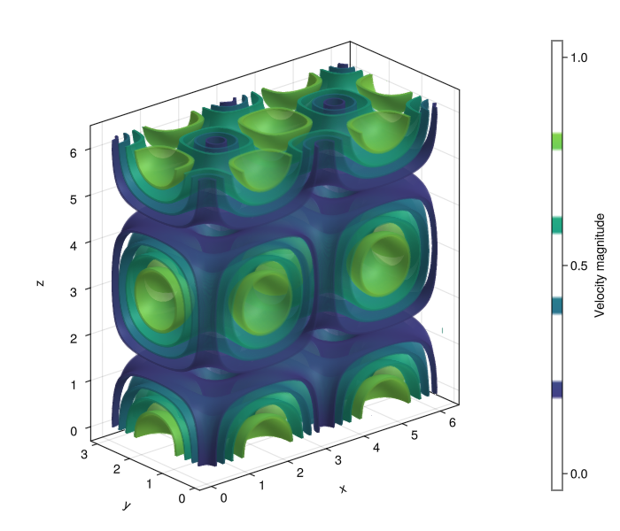

Velocity in Fourier space

In the Fourier pseudo-spectral method, the periodic velocity field is discretised in space as a truncated Fourier series

\[\bm{v}(\bm{x}, t) = ∑_{\bm{k}} \hat{\bm{v}}_{\bm{k}}(t) \, e^{i \bm{k} ⋅ \bm{x}},\]

where $\bm{k} = (k_x, k_y, k_z)$ are the discrete wave numbers.

The wave numbers can be obtained using the fftfreq function. Since we perform a real-to-complex transform along the first dimension, we use rfftfreq instead for $k_x$:

using AbstractFFTs: fftfreq, rfftfreq

ks_global = (
    rfftfreq(Ns[1], 2π * Ns[1] / Ls[1]),  # kx | real-to-complex
     fftfreq(Ns[2], 2π * Ns[2] / Ls[2]),  # ky | complex-to-complex
     fftfreq(Ns[3], 2π * Ns[3] / Ls[3]),  # kz | complex-to-complex
)

ks_global[1]'

1×33 adjoint(::AbstractFFTs.Frequencies{Float64}) with eltype Float64:
 0.0  1.0  2.0  3.0  4.0  5.0  6.0  …  27.0  28.0  29.0  30.0  31.0  32.0

ks_global[2]'

1×64 adjoint(::AbstractFFTs.Frequencies{Float64}) with eltype Float64:
 0.0  1.0  2.0  3.0  4.0  5.0  6.0  …  -6.0  -5.0  -4.0  -3.0  -2.0  -1.0

ks_global[3]'

1×64 adjoint(::AbstractFFTs.Frequencies{Float64}) with eltype Float64:
 0.0  1.0  2.0  3.0  4.0  5.0  6.0  …  -6.0  -5.0  -4.0  -3.0  -2.0  -1.0

To transform the velocity field to Fourier space, we first create a real-to-complex FFT plan to be applied to one of the velocity components:

plan = PencilFFTPlan(v⃗₀[1], Transforms.RFFT())

Transforms: (RFFT, FFT, FFT)
Input type: Float64
Global dimensions: (64, 64, 64) -> (33, 64, 64)
MPI topology: 2D decomposition (2×1 processes)

See PencilFFTPlan for details on creating plans and on optional keyword arguments.

We can now apply this plan to the three velocity components to obtain the respective Fourier coefficients $\hat{\bm{v}}_{\bm{k}}$:

v̂s = plan .* v⃗₀
summary(v̂s[1])

"16×64×64 PencilArray{ComplexF64, 3}(::Pencil{3, 2, Permutation{(3, 2, 1), 3}, Array})"

Note that, in Fourier space, the domain decomposition is performed along the directions $x$ and $y$:

pencil(v̂s[1])

Decomposition of 3D data
    Data dimensions: (33, 64, 64)
    Decomposed dimensions: (1, 2)
    Data permutation: Permutation(3, 2, 1)
    Array type: Array

This is because the 3D FFTs are performed one dimension at a time, with the $x$ direction first and the $z$ direction last. To efficiently perform an FFT along a given direction (taking advantage of serial FFT implementations like FFTW), all the data along that direction must be contained locally within a single MPI process. For that reason, data redistributions (or transpositions) among MPI processes are performed behind the scenes during each FFT computation. Such transpositions require important communications between MPI processes, and are usually the most time-consuming aspect of massively-parallel simulations using this kind of methods.

To solve the Navier–Stokes equations in Fourier space, we will also need the respective wave numbers $\bm{k}$ associated to the local MPI process. Similarly to the local grid points, these are obtained using the localgrid function:

grid_fourier = localgrid(v̂s[1], ks_global)

LocalRectilinearGrid{3} with Permutation(3, 2, 1) and coordinates:
 (1) [0.0, 1.0, 2.0, 3.0, 4.0, 5.0, 6.0, 7.0, 8.0, 9.0, 10.0, 11.0, 12.0, 13.0, 14.0, 15.0]
 (2) [0.0, 1.0, 2.0, 3.0, 4.0, 5.0, 6.0, 7.0, 8.0, 9.0, 10.0, 11.0, 12.0, 13.0, 14.0, 15.0, 16.0, 17.0, 18.0, 19.0, 20.0, 21.0, 22.0, 23.0, 24.0, 25.0, 26.0, 27.0, 28.0, 29.0, 30.0, 31.0, -32.0, -31.0, -30.0, -29.0, -28.0, -27.0, -26.0, -25.0, -24.0, -23.0, -22.0, -21.0, -20.0, -19.0, -18.0, -17.0, -16.0, -15.0, -14.0, -13.0, -12.0, -11.0, -10.0, -9.0, -8.0, -7.0, -6.0, -5.0, -4.0, -3.0, -2.0, -1.0]
 (3) [0.0, 1.0, 2.0, 3.0, 4.0, 5.0, 6.0, 7.0, 8.0, 9.0, 10.0, 11.0, 12.0, 13.0, 14.0, 15.0, 16.0, 17.0, 18.0, 19.0, 20.0, 21.0, 22.0, 23.0, 24.0, 25.0, 26.0, 27.0, 28.0, 29.0, 30.0, 31.0, -32.0, -31.0, -30.0, -29.0, -28.0, -27.0, -26.0, -25.0, -24.0, -23.0, -22.0, -21.0, -20.0, -19.0, -18.0, -17.0, -16.0, -15.0, -14.0, -13.0, -12.0, -11.0, -10.0, -9.0, -8.0, -7.0, -6.0, -5.0, -4.0, -3.0, -2.0, -1.0]

As an example, let's first use this to compute and plot the vorticity associated to the initial condition. The vorticity is defined as the curl of the velocity, $\bm{ω} = \bm{∇} × \bm{v}$. In Fourier space, this becomes $\hat{\bm{ω}} = i \bm{k} × \hat{\bm{v}}$.

using StaticArrays: SVector
using LinearAlgebra: ×

function curl_fourier!(
        ω̂s::NTuple{N, <:PencilArray}, v̂s::NTuple{N, <:PencilArray}, grid_fourier,
    ) where {N}
    @inbounds for I ∈ eachindex(grid_fourier)
        # We use StaticArrays for the cross product between small vectors.
        ik⃗ = im * SVector(grid_fourier[I])
        v⃗ = SVector(getindex.(v̂s, Ref(I)))  # = (v̂s[1][I], v̂s[2][I], ...)
        ω⃗ = ik⃗ × v⃗
        for n ∈ eachindex(ω⃗)
            ω̂s[n][I] = ω⃗[n]
        end
    end
    ω̂s
end

ω̂s = similar.(v̂s)
curl_fourier!(ω̂s, v̂s, grid_fourier);

We finally transform back to physical space and plot the result:

ωs = plan .\ ω̂s

let fig = Figure(size = (700, 600))
    ax = Axis3(fig[1, 1]; aspect = :data, xlabel = "x", ylabel = "y", zlabel = "z")
    ω_norm = parent(vecnorm(ωs))
    ct = contour!(
        ax, to_intervals(grid)..., ω_norm;
        alpha = 0.1, levels = 0.8:0.2:2.0,
        colormap = :viridis, colorrange = (0.8, 2.0),
        highclip = (:red, 0.2), lowclip = (:green, 0.2),
    )
    cb = Colorbar(fig[1, 2], ct; label = "Vorticity magnitude")
    fig
end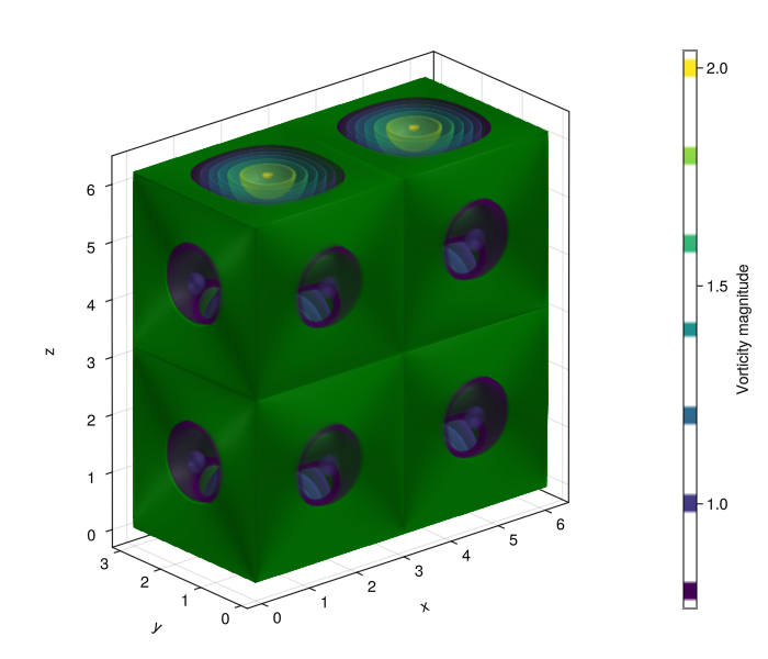

Computing the non-linear term

One can show that, in Fourier space, the incompressible Navier–Stokes equations can be written as

\[∂_t \hat{\bm{v}}_{\bm{k}} = - \mathcal{P}_{\bm{k}} \! \left[ \widehat{(\bm{v} ⋅ \bm{∇}) \bm{v}} \right] - ν |\bm{k}|^2 \hat{\bm{v}}_{\bm{k}} \quad \text{ with } \quad \mathcal{P}_{\bm{k}}(\hat{\bm{F}}_{\bm{k}}) = \left( I - \frac{\bm{k} ⊗ \bm{k}}{|\bm{k}|^2} \right) \hat{\bm{F}}_{\bm{k}},\]

where $\mathcal{P}_{\bm{k}}$ is a projection operator allowing to preserve the incompressibility condition $\bm{∇} ⋅ \bm{v} = 0$. This operator encodes the action of the pressure gradient term, which serves precisely to enforce incompressibility. Note that, because of this, the pressure gradient dissapears from the equations.

Now that we have the wave numbers $\bm{k}$, computing the linear viscous term in Fourier space is straighforward once we have the Fourier coefficients $\hat{\bm{v}}_{\bm{k}}$ of the velocity field. What is slightly more challenging (and much more costly) is the computation of the non-linear term in Fourier space, $\hat{\bm{F}}_{\bm{k}} = \left[ \widehat{(\bm{v} ⋅ \bm{∇}) \bm{v}} \right]_{\bm{k}}$. In the pseudo-spectral method, the quadratic nonlinearity is computed by collocation in physical space (i.e. this term is evaluated at grid points), while derivatives are computed in Fourier space. This requires transforming fields back and forth between both spaces.

Below we implement a function that computes the non-linear term in Fourier space based on its convective form $(\bm{v} ⋅ \bm{∇}) \bm{v} = \bm{∇} ⋅ (\bm{v} ⊗ \bm{v})$. Note that this equivalence uses the incompressibility condition $\bm{∇} ⋅ \bm{v} = 0$.

using LinearAlgebra: mul!, ldiv!  # for applying FFT plans in-place

# Compute non-linear term in Fourier space from velocity field in physical
# space. Optional keyword arguments may be passed to avoid allocations.
function ns_nonlinear!(
        F̂s, vs, plan, grid_fourier;
        vbuf = similar(vs[1]), v̂buf = similar(F̂s[1]),
    )
    # Compute F_i = ∂_j (v_i v_j) for each i.
    # In Fourier space: F̂_i = im * k_j * FFT(v_i * v_j)
    w, ŵ = vbuf, v̂buf
    @inbounds for (i, F̂i) ∈ enumerate(F̂s)
        F̂i .= 0
        vi = vs[i]
        for (j, vj) ∈ enumerate(vs)
            w .= vi .* vj     # w = v_i * v_j in physical space
            mul!(ŵ, plan, w)  # same in Fourier space
            # Add derivative in Fourier space
            for I ∈ eachindex(grid_fourier)
                k⃗ = grid_fourier[I]  # = (kx, ky, kz)
                kj = k⃗[j]
                F̂i[I] += im * kj * ŵ[I]
            end
        end
    end
    F̂s
end

ns_nonlinear! (generic function with 1 method)

As an example, let's use this function on our initial velocity field:

F̂s = similar.(v̂s)
ns_nonlinear!(F̂s, v⃗₀, plan, grid_fourier);

Strictly speaking, computing the non-linear term by collocation can lead to aliasing errors, as the quadratic term excites Fourier modes that fall beyond the range of resolved wave numbers. The typical solution is to apply Orzsag's 2/3 rule to zero-out the Fourier coefficients associated to the highest wave numbers. We define a function that applies this procedure below.

function dealias_twothirds!(ŵs::Tuple, grid_fourier, ks_global)
    ks_max = maximum.(abs, ks_global)  # maximum stored wave numbers (kx_max, ky_max, kz_max)
    ks_lim = (2 / 3) .* ks_max
    @inbounds for I ∈ eachindex(grid_fourier)
        k⃗ = grid_fourier[I]
        if any(abs.(k⃗) .> ks_lim)
            for ŵ ∈ ŵs
                ŵ[I] = 0
            end
        end
    end
    ŵs
end

# We can apply this on the previously computed non-linear term:
dealias_twothirds!(F̂s, grid_fourier, ks_global);

Finally, we implement the projection associated to the incompressibility condition:

function project_divergence_free!(ûs, grid_fourier)
    @inbounds for I ∈ eachindex(grid_fourier)
        k⃗ = grid_fourier[I]
        k² = sum(abs2, k⃗)
        iszero(k²) && continue  # avoid division by zero
        û = getindex.(ûs, Ref(I))  # (ûs[1][I], ûs[2][I], ...)
        for i ∈ eachindex(û)
            ŵ = û[i]
            for j ∈ eachindex(û)
                ŵ -= k⃗[i] * k⃗[j] * û[j] / k²
            end
            ûs[i][I] = ŵ
        end
    end
    ûs
end

project_divergence_free! (generic function with 1 method)

We can verify the correctness of the projection operator by checking that the initial velocity field is not modified by it, since it is already incompressible:

v̂s_proj = project_divergence_free!(copy.(v̂s), grid_fourier)
v̂s_proj .≈ v̂s  # the last one may be false because v_z = 0 initially

(true, true, false)

Putting it all together

To perform the time integration of the Navier–Stokes equations, we will use the timestepping routines implemented in the DifferentialEquations.jl suite. For simplicity, we use here an explicit Runge–Kutta scheme. In this case, we just need to write a function that computes the right-hand side of the Navier–Stokes equations in Fourier space:

function ns_rhs!(
        dvs::NTuple{N, <:PencilArray}, vs::NTuple{N, <:PencilArray}, p, t,
    ) where {N}
    # 1. Compute non-linear term and dealias it
    (; plan, cache, ks_global, grid_fourier) = p
    F̂s = cache.F̂s
    ns_nonlinear!(F̂s, vs, plan, grid_fourier; vbuf = dvs[1], v̂buf = cache.v̂s[1])
    dealias_twothirds!(F̂s, grid_fourier, ks_global)

    # 2. Project onto divergence-free space
    project_divergence_free!(F̂s, grid_fourier)

    # 3. Transform velocity to Fourier space
    v̂s = cache.v̂s
    map((v, v̂) -> mul!(v̂, plan, v), vs, v̂s)

    # 4. Add viscous term (and multiply projected non-linear term by -1)
    ν = p.ν
    for n ∈ eachindex(v̂s)
        v̂ = v̂s[n]
        F̂ = F̂s[n]
        @inbounds for I ∈ eachindex(grid_fourier)
            k⃗ = grid_fourier[I]  # = (kx, ky, kz)
            k² = sum(abs2, k⃗)
            F̂[I] = -F̂[I] - ν * k² * v̂[I]
        end
    end

    # 5. Transform RHS back to physical space
    map((dv, dv̂) -> ldiv!(dv, plan, dv̂), dvs, F̂s)

    nothing
end

ns_rhs! (generic function with 1 method)

For the time-stepping, we load OrdinaryDiffEq.jl from the DifferentialEquations.jl suite and set-up the simulation. Since DifferentialEquations.jl can't directly deal with tuples of arrays, we convert the input data to the ArrayPartition type and write an interface function to make things work with our functions defined above.

using OrdinaryDiffEqLowOrderRK  # includes RK4
using RecursiveArrayTools: ArrayPartition

ns_rhs!(dv::ArrayPartition, v::ArrayPartition, args...) = ns_rhs!(dv.x, v.x, args...)
vs_init_ode = ArrayPartition(v⃗₀)
summary(vs_init_ode)

"RecursiveArrayTools.ArrayPartition{Float64, Tuple{PencilArray{Float64, 3, Array{Float64, 3}, 3, 0, Pencil{3, 2, NoPermutation, Vector{UInt8}}}, PencilArray{Float64, 3, Array{Float64, 3}, 3, 0, Pencil{3, 2, NoPermutation, Vector{UInt8}}}, PencilArray{Float64, 3, Array{Float64, 3}, 3, 0, Pencil{3, 2, NoPermutation, Vector{UInt8}}}}} with arrays:"

We now define solver parameters and temporary variables, and initialise the problem:

params = (;
    ν = 5e-3,  # kinematic viscosity
    plan, grid_fourier, ks_global,
    cache = (
        v̂s = similar.(v̂s),
        F̂s = similar.(v̂s),
    )
)

tspan = (0.0, 10.0)
prob = ODEProblem{true}(ns_rhs!, vs_init_ode, tspan, params)
integrator = init(prob, RK4(); dt = 1e-3, save_everystep = false);

We finally solve the problem over time and plot the vorticity associated to the solution. It is also useful to look at the energy spectrum $E(k)$, to see if the small scales are correctly resolved. To obtain a turbulent flow, the viscosity $ν$ must be small enough to allow the transient appearance of an energy cascade towards the small scales (i.e. from small to large $k$), while high enough to allow the small-scale motions to be correctly resolved.

function energy_spectrum!(Ek, ks, v̂s, grid_fourier)
    Nk = length(Ek)
    @assert Nk == length(ks)
    Ek .= 0
    for I ∈ eachindex(grid_fourier)
        k⃗ = grid_fourier[I]  # = (kx, ky, kz)
        knorm = sqrt(sum(abs2, k⃗))
        i = searchsortedfirst(ks, knorm)
        i > Nk && continue
        v⃗ = getindex.(v̂s, Ref(I))  # = (v̂s[1][I], v̂s[2][I], ...)
        factor = k⃗[1] == 0 ? 1 : 2  # account for Hermitian symmetry and r2c transform
        Ek[i] += factor * sum(abs2, v⃗) / 2
    end
    MPI.Allreduce!(Ek, +, get_comm(v̂s[1]))  # sum across all processes
    Ek
end

ks = rfftfreq(Ns[1], 2π * Ns[1] / Ls[1])
Ek = similar(ks)
v̂s = plan .* integrator.u.x
energy_spectrum!(Ek, ks, v̂s, grid_fourier)
Ek ./= scale_factor(plan)^2  # rescale energy

curl_fourier!(ω̂s, v̂s, grid_fourier)
ldiv!.(ωs, plan, ω̂s)
ω⃗_plot = Observable(ωs)
k_plot = @view ks[2:end]
E_plot = Observable(@view Ek[2:end])
t_plot = Observable(integrator.t)

fig = let
    fig = Figure(size = (1200, 600))
    ax = Axis3(
        fig[1, 1][1, 1]; title = @lift("t = $(round($t_plot, digits = 3))"),
        aspect = :data, xlabel = "x", ylabel = "y", zlabel = "z",
    )
    ω_mag = @lift parent(vecnorm($ω⃗_plot))
    ω_mag_norm = @lift $ω_mag ./ maximum($ω_mag)
    ct = contour!(
        ax, to_intervals(grid)..., ω_mag_norm;
        alpha = 0.3, levels = 3,
        colormap = :viridis, colorrange = (0.0, 1.0),
        highclip = (:red, 0.2), lowclip = (:green, 0.2),
    )
    cb = Colorbar(fig[1, 1][1, 2], ct; label = "Normalised vorticity magnitude")
    ax_sp = Axis(
        fig[1, 2];
        xlabel = "k", ylabel = "E(k)", xscale = log2, yscale = log10,
        title = "Kinetic energy spectrum",
    )
    ylims!(ax_sp, 1e-8, 1e0)
    scatterlines!(ax_sp, k_plot, E_plot)
    ks_slope = exp.(range(log(2.5), log(25.0), length = 3))
    E_fivethirds = @. 0.3 * ks_slope^(-5/3)
    @views lines!(ax_sp, ks_slope, E_fivethirds; color = :black, linestyle = :dot)
    text!(ax_sp, L"k^{-5/3}"; position = (ks_slope[2], E_fivethirds[2]), align = (:left, :bottom))
    fig
end

record(fig, "vorticity_proc$procid.mp4"; framerate = 10) do io
    while integrator.t < 20
        dt = 0.001
        step!(integrator, dt)
        t_plot[] = integrator.t
        mul!.(v̂s, plan, integrator.u.x)  # current velocity in Fourier space
        curl_fourier!(ω̂s, v̂s, grid_fourier)
        ldiv!.(ω⃗_plot[], plan, ω̂s)
        ω⃗_plot[] = ω⃗_plot[]  # to force updating the plot
        energy_spectrum!(Ek, ks, v̂s, grid_fourier)
        Ek ./= scale_factor(plan)^2  # rescale energy
        E_plot[] = E_plot[]
        recordframe!(io)
    end
end;

This page was generated using Literate.jl.